In the previous article, I have described a few evolution strategies (ES) algorithms that can optimise the parameters of a function without the need to explicitly calculate gradients. These algorithms can be applied to reinforcement learning (RL) problems to help find a suitable set of model parameters for a neural network agent. In this article, I will explore applying ES to some of these RL problems, and also highlight methods we can use to find policies that are more stable and robust.

Evolution Strategies for Reinforcement Learning

While RL algorithms require a reward signal to be given to the agent at every timestep, ES algorithms only care about the final cumulative reward that an agent gets at the end of its rollout in an environment. In many problems, we only know the outcome at the end of the task, such as whether the agent wins or loses, whether the robot arm picks up the object or not, or whether the agent has survived, and these are problems where ES may have an advantage over traditional RL. Below is a pseudo-code that encapsulates a rollout of an agent in an OpenAI Gym environment, where we only care about the cumulative reward:

def rollout(agent, env):
  obs = env.reset()
  done = False
  total_reward = 0
  while not done:
    a = agent.get_action(obs)
    obs, reward, done = env.step(a)
    total_reward += reward
  return total_reward

We can define rollout to be the objective function that maps the model parameters of an agent into its fitness score, and use an ES solver to find a suitable set of model parameters as described in the previous article:

env = gym.make('worlddomination-v0')

# use our favourite ES
solver = EvolutionStrategy()

while True:

  # ask the ES to give set of params
  solutions = solver.ask()

  # create array to hold the results
  fitlist = np.zeros(solver.popsize)

  # evaluate for each given solution
  for i in range(solver.popsize):

    # init the agent with a solution
    agent = Agent(solutions[i])

    # rollout env with this agent
    fitlist[i] = rollout(agent, env)

  # give scores results back to ES
  solver.tell(fitness_list)

  # get best param & fitness from ES
  bestsol, bestfit = solver.result()

  # see if our task is solved
  if bestfit > MY_REQUIREMENT:
    break

Deterministic and Stochastic Policies

Our agent takes the observation given to it by the environment as an input, and outputs an action at each timestep during a rollout inside the environment. We can model the agent however we want, and use methods from hard-coded rules, decision trees, linear functions to recurrent neural networks. In this article I use a simple feed-forward network with 2 hidden layers to map from an agent’s observation, a vector $x$, directly to the actions, a vector $y$:

The activation functions $f_h$, $f_{out}$ can be tanh, sigmoid, relu, or whatever we want to use. In all of my experiments I use tanh. For the output layer, sometimes we may want $f_{out}$ to be a pass-through function without nonlinearities. If we concatenate all the weight and bias parameters into a single vector called $W$, we see that the above neural network is a deterministic function $y = F(x, W)$. We can then use ES to find a solution $W$ using the search loop described earlier.

But what if we don’t want our agent’s policy to be deterministic? For certain tasks, even as simple as rock-paper-scissors, the optimal policy is a random action, so we want our agent to be able to learn a stochastic policy. One way to convert $y=F(x, W)$ into a stochastic policy is to make $W$ random. Each model parameter $w_i \in W$ can be a random value drawn from a normal distribution $N(\mu_i, \sigma_i)$.

This type of stochastic network is called a Bayesian Neural Network. A Bayesian neural network is a neural network with a prior distribution on its weights. In this case, the model parameters we want to solve for, are the set of $\mu$ and $\sigma$ vectors, rather than the weights $W$. During each forward pass of the network, a new $W$ is drawn from $N(\mu, \sigma I)$. There are lots of interesting works in the literature applying Bayesian networks to many problems, and also addressing many challenges of training these networks. ES can also be used to directly find solutions for a stochastic policy by setting the solutions space be $\mu$ and $\sigma$, rather than $W$.

Stochastic policy networks are also popular in the RL literature. For example, in the Proximal Policy Optimization (PPO) algorithm, the final layer is a set of $\mu$ and $\sigma$ parameters and the action is sampled from $N(\mu, \sigma I)$. Adding noise to parameters are also known to encourage the agent to explore the environment and escape from local optima. I find that for many tasks where we need an agent to explore, we do not need the entire $W$ to be random – just the bias is enough. For challenging locomotion tasks, such as the ones in the roboschool environment, I often need to use ES to find a stochastic policy where only the bias parameters are drawn from a normal distribution.

Evolving Robust Policies for Bipedal Walker

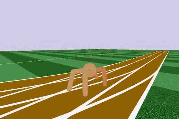
One of the areas where I found ES useful is for searching for robust policies. I want to control the tradeoff between data efficiency, and how robust the policy is over several random trials. To demonstrate this, I tested ES on a nice environment called BipedalWalkerHardcore-v2 created by Oleg Klimov using the Box2D Physics Engine, the same physics engine used in Angry Birds.

In this environment our agent has to learn a policy to walk across randomly generated terrain within the time limit without falling over. There are 24 inputs, consisting of 10 lidar sensors, angles and contacts. The agent is not given the absolute coordinates of where it is on the map. The action space is 4 continuous values controlling the torques of its 4 motors. The total reward calculation is based on the total distance achieved by the agent. Generally, if the agent completes a map, it will get score of 300+ points, although a small amount of points will be subtracted based on how much motor torque was applied, so energy usage is also a constraint.

BipedalWalkerHardcore-v2 defines solving the task as getting an average score of 300+ over 100 consecutive random trials. While it is relatively easy to train an agent to successfully walk across the map using an RL algorithm, it is difficult to get the agent to do so consistently and efficiently, making this task an interesting challenge. To my knowledge, my agent is the only solution known to solve this task so far (as of October 2017).

Early stages. Learning to walk.

Learns to correct errors, but still slow ...

Because the terrain map is randomly generated for each trial, sometimes we may end up with an easy terrain, or sometimes a very difficult terrain. We don’t want our natural selection process to allow agents with weak policies who had gotten lucky with an easy map to advance to the next generation. We also want to give agents with good policies a chance to redeem themselves. So what I ended up doing, is to define an agent’s episode, as the average of 16 random rollouts, and use the average of the cumulative rewards over 16 rollouts as its fitness score.

Another way to look at this is to see that even though we are testing the agent over 100 trials, we usually train it on single trials, so the test-task is not the same as the training-task we are optimising for. By averaging each agent in the population multiple times in a stochastic environment, we narrow the gap between our training set and the test set. If we can overfit to the training set, we might as well overfit to the test set, since that’s an okay thing to do in RL :)

Of course, the data efficiency of our algorithm is now 16x worse, but the final policy is a lot more robust. When I tested the final policy over 100 consecutive random trials, we got an average score of over 300 points required to solve this environment. Without this averaging method, the best agent can only obtain an average score of $\sim$ 220 to 230 over 100 trials. To my knowledge, this is the first solution that solves this environment (as of October 2017).

Winning solutions evolved using PEPG using average-of-16 runs per episode.

I also used PPO, a state-of-the-art policy gradient algorithm for RL, and tried to tune it to the best of my ability to perform well on this task. In the end, I was only able to get PPO to achieve average scores of $\sim$ 240 to 250 over 100 random trials. But I’m sure someone else will be able to use PPO or another RL algorithm to solve this environment in the future. (Please let me know if you do so!)

Update (Jan 2018): dgriff777 was able to use a continuous version of A3C+LSTM with 4 stack frames as the input to train BipedalWalkerHardcore-v2 to obtain a score of 300 over 100 random trials. He provided this awesome implementation of his pytorch model on GitHub.

The ability to control the tradeoff between data efficiency and policy robustness is quite powerful, and useful in the real world where we need safe policies. In theory, with enough compute, we could have even averaged over of the required 100 rollouts and optimised our Bipedal Walker directly to the requirements. Professional engineers are often required to have their designs satisfy specific Quality Assurance guarantees and meet certain safety factors. We need to be able to take into account such safety factors when we train agents to learn policies that may affect the real world.

Here are a few other solutions that ES discovered:

CMA-ES solution

OpenAI-ES solution

I also trained the agent with a stochastic policy network with high initial noise parameters, so the agent sees noise everywhere, and even its actions are noisy. It resulted in the agent learning the task despite not being confident of its input and outputs being accurate (this agent couldn’t get a score of 300+ though):

Bipedal walker using a stochastic policy.

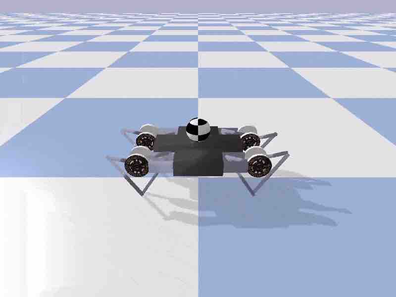
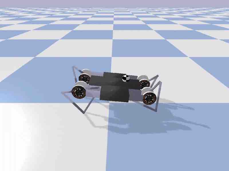
Kuka Robot Arm Grasping

I also tried to apply ES with this averaging technique on a simplified Kuka robot arm grasping task. This environment is available in the pybullet environment. The Kuka model used in the simulation is designed to be similar to a real Kuka robot arm. In this simplified task, the agent is given the coordinates of the object.

More advanced RL environments may require the agent to infer an action directly from pixel inputs, but we could in principle combine this simplified model with a pre-trained convnet that gives us an estimate of the coordinates as well.

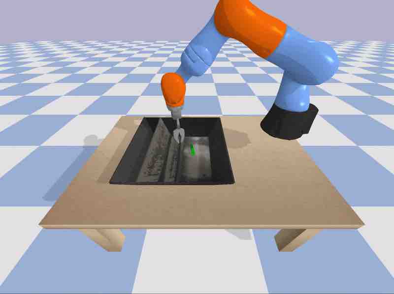
Robot arm grasping task using a stochastic policy.

The agent obtains a score of 10000 if it successfully picks up the object, and 0 otherwise. Some points are deducted for energy usage. By averaging a sparse reward over 16 random trials, we can get the ES to optimise for robustness. However, in the end, I was able to get policies that can pick up the object only $\sim$ 70 to 75% of the time with both deterministic and stochastic policies. There is still room for improvement.

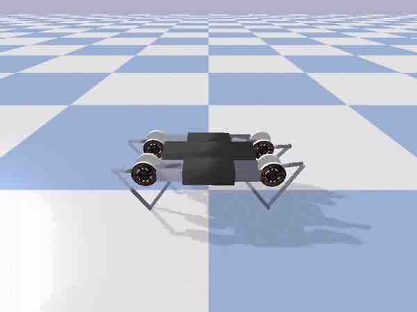
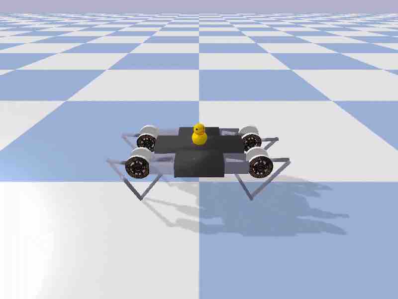
Getting a Minitaur to Learn a Multiple Tasks

Learning to perform multiple difficult tasks at the same time make us better at performing individual tasks. For example, Shaolin monks who lift weights while standing on a pole will be able to balance better without the weights. Learning to not spill a cup of water while cruising a car at 80mph in the mountains will make the driver a better illegal street racer. We can also train agents to perform multiple tasks to make them learn more stable policies.

Shaolin Agents.

Learning to drift.

This recent work on self-playing agents demonstrated that agents who learn difficult tasks such as Sumo wrestling (a sport that require many skills) are able to also perform easier tasks, like withstanding wind while walking, without the need for further training. Erwin Coumans recently tried to experiment with adding a duck on top of a Minitaur learning to walk ahead. If the duck fell, the Minitaur would also fail, so the hope is that these types of task augmentation will help transfer learned policies from simulation over to the real Minitaur. I took one of his examples and experimented with training the Minitaur and duck combination using ES.

CMA-ES walking policy in pybullet.

Real Minitaur from Ghost Robotics.

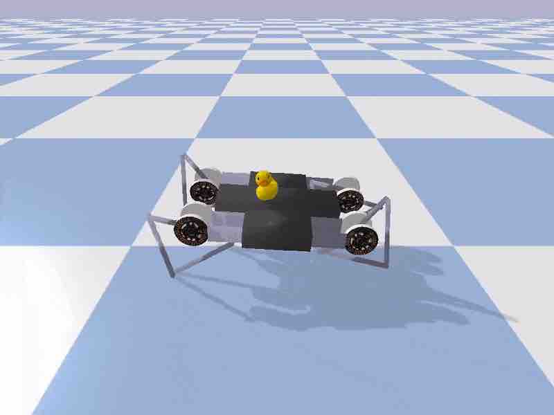
The Minitaur model in pybullet is designed to mimic the real physical Minitaur. However, a policy trained on a perfect simulation environment usually fails in the real world. It may not even generalise to small augmentations of the task inside the simulation. For example, in the figure above is a Minitaur trained to walk ahead (using CMA-ES), but we see that this policy is not always able to carry a duck across the room when we put a duck on top of it inside of the simulation.

Walking policy works with duck.

Policy trained on duck.

The policy learned from the pure walking task still works to some degree even when the duck is deployed, meaning that the addition of the duck wasn’t so difficult. The duck has a flat stable bottom so it wasn’t too difficult for the Minitaur to keep the duck from falling off its back. I tried to replace the duck with a ball to make the task much harder.

Learning to cheat.

However, replacing the duck with a ball didn’t immediately result in a stable balancing policy. Instead, CMA-ES found a policy that still technically carried the ball across the floor by first having the ball slide into a hole made for its legs, and then carrying the ball inside this hole. The lesson learned here is that an objective-driven search algorithm will learn to take advantage of any design flaws in the environment and exploit them to reach its objective.

Stochastic policy trained with ball.

Same policy with duck.

After making the ball smaller, CMA-ES was able to find a stochastic policy that can walk and balance the ball at the same time. This policy also transferred back to the easier duck task. In the future, I hope these type of task augmentation techniques will be useful for transfer learning to real robots.

ESTool

One of the big selling points of ES is that it is easy to parallelise the computation using several workers running on different threads on different CPU cores, or even on different machines. Python’s multiprocessing makes it simple to launch parallel processes. I prefer to use Message Passing Interface (MPI) with mpi4py to launch separate python processes for each job. This allows us to get around the global interpreter lock, and also gives me confidence that each process has its own sandboxed numpy and gym instances which is important when it comes to seeding random number generators.

Roboschool Hopper, Walker, Ant.

Roboschool Reacher.

Agents evolved using estool on various roboschool tasks.

I have implemented a simple tool called estool that uses the es.py library described in the previous article to train simple feed-forward policy networks to perform continuous control RL tasks written with a gym interface. I have used estool tool to easily train all of the experiments described earlier, as well as various other continuous control tasks inside gym and roboschool. estool uses MPI for distributed processing so it shouldn’t require too much work to distribute workers over multiple machines.

ESTool with pybullet

GitHub repo

In addition to the environments that come with gym and roboschool, estool works well with most pybullet gym environments. It is also easy to build custom pybullet environments by modifying existing environments. For example, I was able to make the Minitaur with ball environment (in the custom_envs directory of the repo) without much effort, and being able to tinker with the environment makes it easier to try out new ideas. If you want to incorporate 3D models from other software packages like ROS or Blender, you can try building new and interesting pybullet environments and challenge others to try to solve them.

Many models and environments in pybullet, such as the Kuka robot arm and the Minitaur, are modelled to be similar to the real robot as part of current exciting transfer learning research efforts. In fact, many of these recent cutting edge research papers are using pybullet to conduct transfer learning experiments.

You don’t need an expensive Minitaur or Kuka robot arm to play with sim-to-real experiments though. There is a racecar model inside pybullet that is modelled after the MIT racecar open source hardware kit. There’s even a pybullet environment that mounts a virtual camera onto the virtual racecar to give the agent a virtual pixel screen as an input observation.

Let’s try the easier version first, where the racecar simply needs to learn a policy to move towards a giant ball. In the RacecarBulletEnv-v0 environment, the agent gets the relative coordinates of the ball as an input, and outputs continuous actions that control the motor speed and steering direction. The task is simple enough that it only takes 5 minutes (50 generations) on a 2014 Macbook Pro (with an 8-core CPU) to train. Using estool, the command below will launch the training job on eight processes and assign each process 4 jobs, to get a total of 32 workers, using CMA-ES to evolve the policies:

python train.py bullet_racecar -o cma -n 8 -t 4

The training progress, as well as the model parameters found will be stored in the log subdirectory. We can run this command to visualise an agent inside the environment using the best policy found:

python model.py bullet_racecar log/bullet_racecar.cma.1.32.best.json

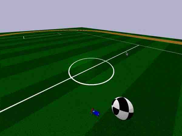
pybullet racecar environment, based on the MIT Racecar.

In the simulation, we can use the mouse cursor to move the ball around, and even move the racecar around if we want to interact with it.

The IPython notebook plot_training_progress.ipynb can visualise the training history per generation of the racecar agents. At each generation, we can see the best score, the worse score, and the average score across the entire population.

Standard locomotion tasks similar to those in roboschool, such as Inverted Pendulum, Hopper, Walker, HalfCheetah, Ant, and Humanoid are also available in pybullet. I found a policy for pybullet’s ant that gets to a score of 3000 within hours on a multi-core machine with a population size of 256, using PEPG:

python train.py bullet_ant -o pepg -n 64 -t 4

Example rollout of AntBulletEnv. We can still save rollouts as an .mp4 video using gym.wrappers.Monitor

Summary

In this article, I discussed using ES to find policies for a feed-forward neural network agent to perform various continuous control RL tasks defined by a gym environment interface. I described the estool that allowed me to quickly try different ES algorithms with various settings in a distributed processing environment using the MPI framework.

So far, I have only discussed methods for training an agent by having it learn a policy from trial-and-error in the environment. This form of training from scratch is referred to as model-free reinforcement learning. In the next article (if I ever get to writing it), I will discuss more about model-based learning, where our agent will learn to exploit a previously learned model to accomplish a given task. And yes, I will still be using evolution.

Citation

If you find this work useful, please cite it as:

@article{ha2017evolving,
  title   = "Evolving Stable Strategies",
  author  = "Ha, David",
  journal = "blog.otoro.net",
  year    = "2017",
  url     = "https://blog.otoro.net/2017/11/12/evolving-stable-strategies/"
}

Acknowledgements

I want to thank Erwin Coumans for writing all these great environments, and also for helping me work on making ESTool better. Great research cannot be done without great tools.

In the end, it all comes to choices to turn stumbling blocks into stepping stones.

Interesting Links

“Fires of a Revolution” Incredible Fast Piano Music (EPIC)

A Visual Guide to Evolution Strategies

ESTool

Stable or Robust? What’s the Difference?

OpenAI Gym Docs

Evolution Strategies as a Scalable Alternative to Reinforcement Learning

Edward, A library for probabilistic modeling, inference, and criticism

History of Bayesian Neural Networks

BipedalWalkerHardcore-v2

roboschool

pybullet

Emergent Complexity via Multi-Agent Competition

GraspGAN