GitHub
In this article I will give step-by-step instructions for reproducing the experiments in the World Models article (pdf). The reference TensorFlow implementation is on GitHub.
Other people have implemented World Models independently. There is an implementation in Keras that reproduces part of the CarRacing-v0 experiment. There is also another project in PyTorch that attempts to apply this model on OpenAI Retro Sonic environments.
For general discussion about the World Models article, there are already some good discussion threads here in the GitHub issues page of the interactive article. If you have any issues specific to the code, please don’t hessitate to raise an issue to discuss.
Pre-requisite reading
I recommend reading the following articles to gain some background knowledge before attempting to reproduce the experiments.
A Visual Guide to Evolution Strategies
Below is optional
Mixture Density Networks with TensorFlow
Read tutorials on Variational Autoencoders if you are not familiar with them. Some Examples:
Variational Autoencoder in TensorFlow
Building Autoencoders in Keras
Generating Large Images from Latent Vectors.
Be familiar with RNNs for continuous sequence generation:
Generating Sequences With Recurrent Neural Networks
A Neural Representation of Sketch Drawings
Handwriting Generation Demo in TensorFlow
Recurrent Neural Network Tutorial for Artists.
Software Settings
I have tested the code with the following settings:
- Ubuntu 16.04
- Python 3.5.4
- TensorFlow 1.8.0
- NumPy 1.13.3
- VizDoom Gym Levels
(Latest commit 60ff576 on Mar 18, 2017) - OpenAI Gym 0.9.4 (Note: Gym 1.0+ breaks this experiment. Only tested for 0.9.x)
- cma 2.2.0
- mpi4py 2, see estool, which we have forked for this project.
- Jupyter Notebook for model testing, and tracking progress.
I use a combination of OS X for inference, but trained models using Google Cloud VMs. I trained the V and M models on a P100 GPU instance, but trained the controller C on pure CPU instance with 64 cpu-cores (n1-standard-64) using CMA-ES. I will outline which part of the training requires GPUs and which parts use only CPUs, and try to keep your costs low for running this experiment.
Instructions for running pre-trained models
You only need to clone the repo into your desktop computer running in CPU-mode to reproduce the results with pre-trained models provided in the repo. No Clould VM or GPUs necessary.
CarRacing-v0
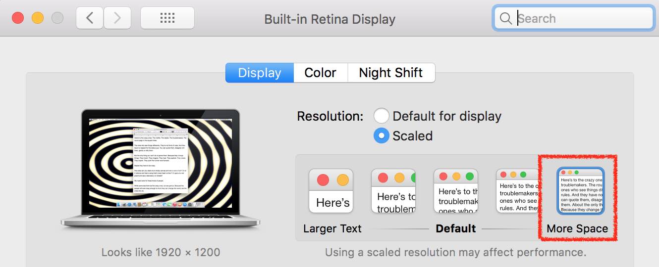
If you are using a MacBook Pro, I recommend setting the resolution to “More Space”, since the CarRacing-v0 environment renders at a larger resolution and doesn’t fit in the default screen settings.
In the command line, go into the carracing subdirectory. Try to play the game yourself, run python env.py in a terminal. You can control the car using the four arrow keys on the keyboard. Press (up, down) for accelerate/brake, and (left/right) for steering.
In this environment, a new random track is generated for each run. While I can consistently get above 800 if I drive very carefully, it is hard for me to consistently get a score above 900 points. Some Stanford students also found it tough to get consistently higher than 900. The requirement to solve this environment is to obtain an average score of 900 over 100 consecutive random trails.
To run the pre-trained model once and see the agent in full-rendered mode, run:
python model.py render log/carracing.cma.16.64.best.json
Run the pre-trained model 100 times in no-render mode (in no-render mode, it still renders something simpler on the screen due to the need to use OpenGL for this environment to extract the pixel information as observations):
python model.py norender log/carracing.cma.16.64.best.json
This command will output the score for each 100 trials, and after running 100 times. It will also output the average score and standard deviation. The average score should be above 900.
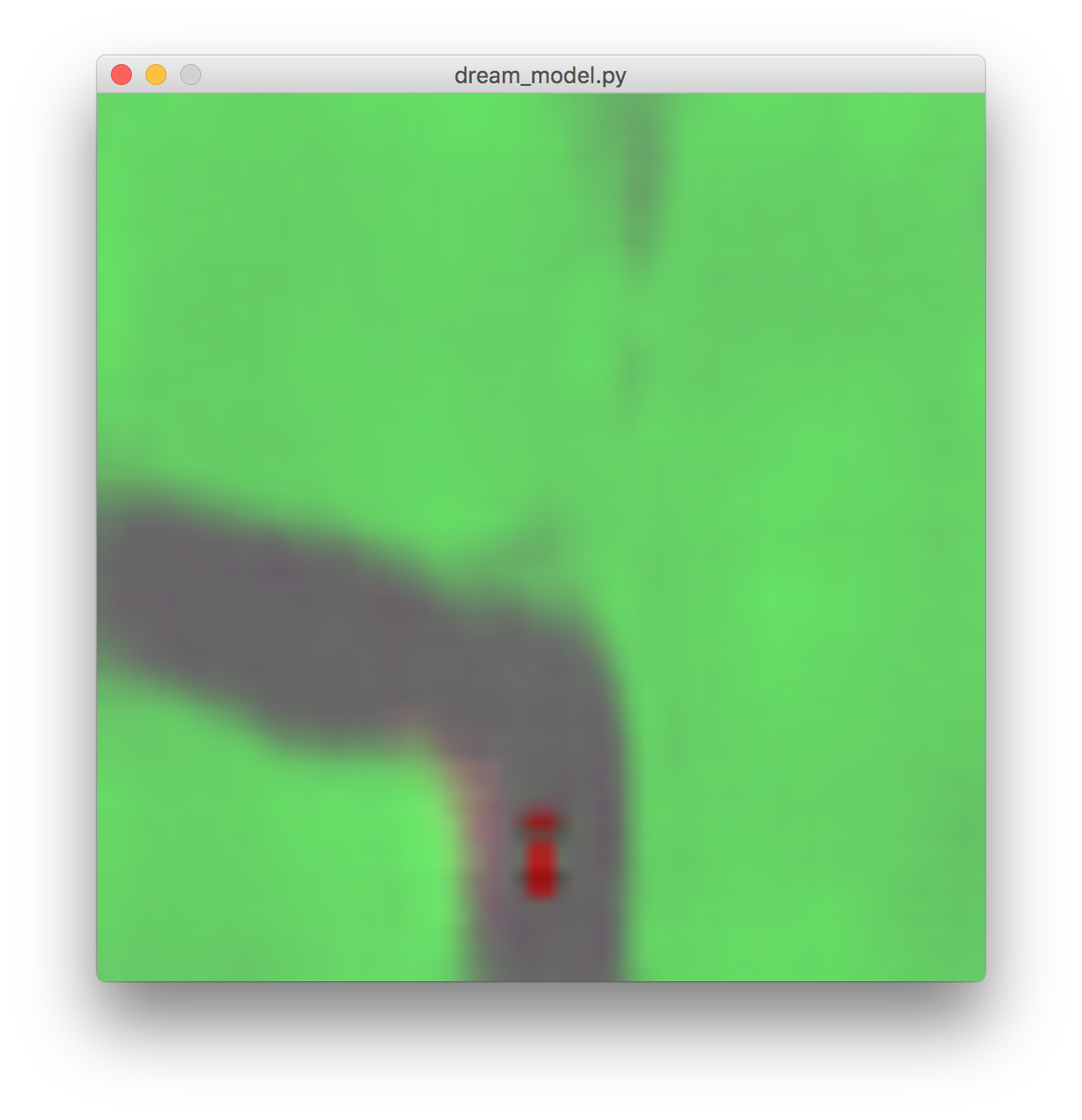
To run the pre-trained controller inside of an environment generated using M and visualized using V:
python dream_model.py log/carracing.cma.16.64.best.json
DoomTakeCover-v0
In the doomrnn directory, run python doomrnn.py to play inside of an environment generated by M.
You can hit left, down, or right to play inside of this envrionment. To visualize the pre-trained model playing inside of the real environment, run:
python model.py doomreal render log/doomrnn.cma.16.64.best.json
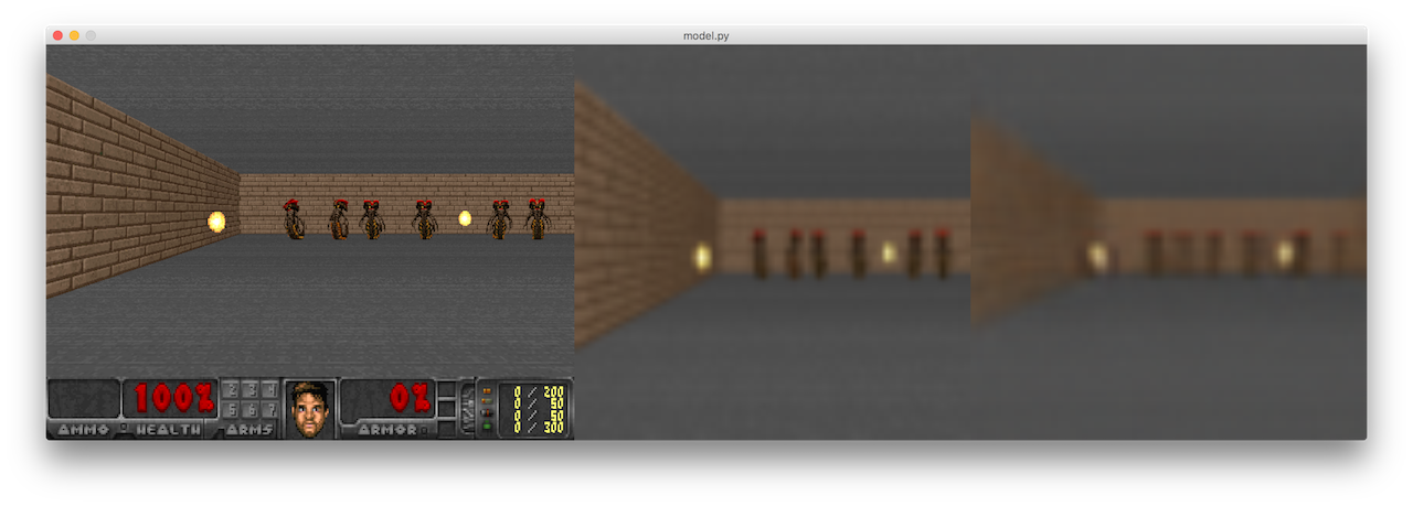
Note that this environment is modified to also display the cropped 64x64px frames, in addition to the reconstructed frames and actual frames of the game. To run model inside the actual environment 100 times and compute the mean score, run:
python model.py doomreal norender log/doomrnn.cma.16.64.best.json
You should get a mean score of over 900 time-steps over 100 random episodes. The above two lines still work if you substitute doomreal with doomrnn if you want to get the statistics of the agent playing inside of the generated environment. If you wish to change the temperature of the generated environment, modify the constant TEMPERATURE inside doomrnn.py, which is currently set to 1.25.
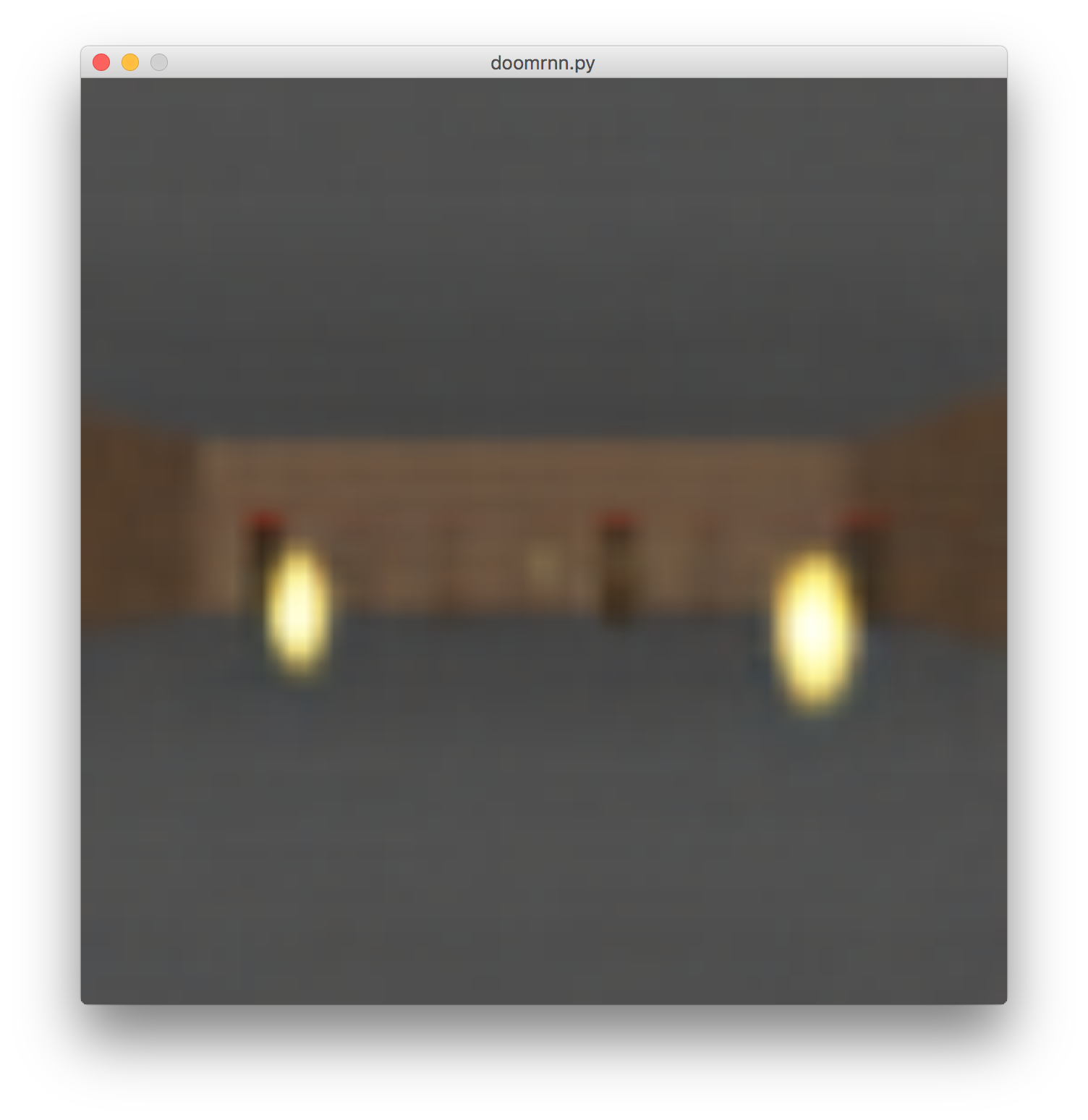
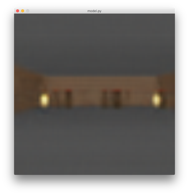
To visualie the model playing inside of the generated environment, run:
python model.py doomrnn render log/doomrnn.cma.16.64.best.json
Instructions for training everything from scratch
The DoomTakeCover-0 experiment should take less than 24 hours to completely reproduce from scratch using a P100 instance and 64-core CPU instance on Google Cloud Platform.
DoomTakeCover-v0
I will discuss the VizDoom experiment first since it requires less compute time to reproduce from scratch. Since you may update the models in the repo, I recommend that you fork the repo and clone/update on your fork. I recommend running any command inside of a tmux session so that you can close your ssh connections and the jobs will still run on the background.
I first create a 64-core CPU instance with ~ 200GB storage and 220GB RAM, and clone the repo in that instance. In the doomrnn directory, there is a script called extract.py that will extract 200 episodes from a random poilcy, and save the episodes as .npz files in doomrnn/record. A bash script called extract.bash will run extract.py 64 times (~ one job per CPU core), so by running bash extract.bash, we will generate 12,800 .npz files in doomrnn/record. Some instances might randomly fail, so we generate a bit of extra data, although in the end we only use 10,000 episodes for training V and M. This process will take a few hours (probably less than 5 hours).
After the .npz files have been created in the record subdirectory, I create a P100 GPU instance with ~ 200GB storage and 220GB RAM, and clone the repo there too. I use the ssh copy command, scp, to copy all of the .npz files from the CPU instance to the GPU instance, into the same record subdirectory. You can use the gcloud tool if scp doesn’t work. This should be really fast, like less than a minute, if both instances are in the same region. Shut down the CPU instance after you have copied the .npz files over to the GPU machine.
On the GPU machine, run the command bash gpu_jobs.bash to train the VAE, pre-process the recorded dataset, and train the MDN-RNN.
This gpu_jobs.bash will run 3 things in sequential order:
1) python vae_train.py - which will train the VAE, and after training, the model will be saved in tf_vae/vae.json
2) Next, it will pre-process collected data using pre-trained VAE by launching: python series.py. A new dataset will be created in a subdirectory called series.
3) After this a series.npz dataset is saved there, the script will launch the MDN-RNN trainer using this command: python rnn_train.py. This will produce a model in tf_rnn/rnn.json and also tf_initial_z/initial_z.json. The file initial_z.json saves the initial latent variables (z) of an episode which is needed when we need to generate the environment. This entire process might take 6-8 hours.
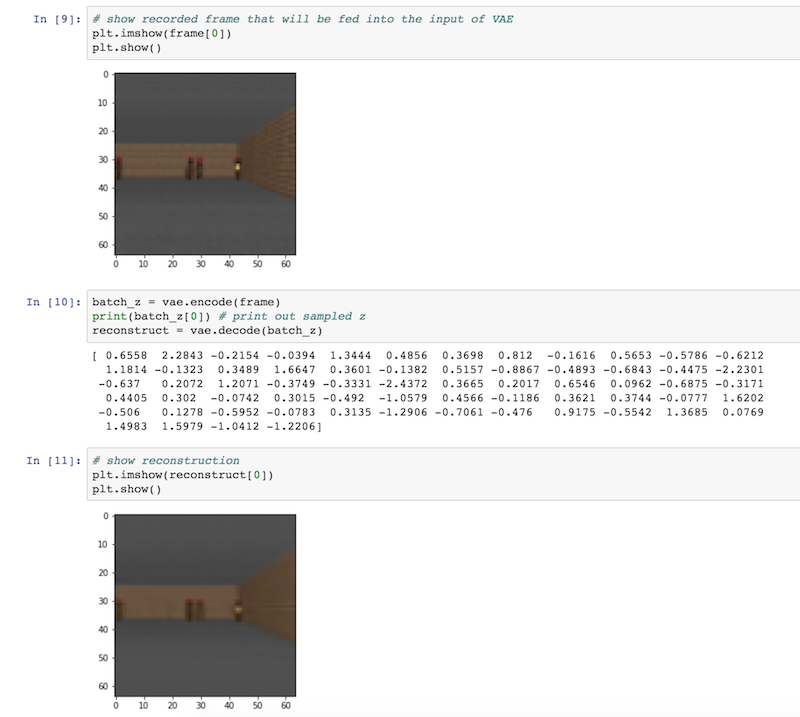
The notebook
vae_test.ipynb will visualize input/reconstruction images using your VAE on the training dataset.
After V and M are trained, and you have the 3 new json files, you must must now copy vae.json, initial_z.json and rnn.json over to tf_models subdirectory and overwrite previous files that might be there. You should update your git repo with these new models using git add doomrnn/tf_models/*.json and committing the change to your fork. After you have done this, you can shutdown the GPU machine. You need to start the 64-core CPU instance again, log back into that machine.
Now on a 64-core CPU instance, run the CMA-ES based training by launching the command: python train.py inside the doomrnn directory. This will launch the evolution trainer and continue training until you Ctrl-C this job. The controller C will be trained inside of M’s generated environment with a temperature of 1.25. You can monitor progress using the plot_training_progress.ipynb notebook which loads the log files being generated. After 200 generations (or around 4-5 hours), it should be enough to get decent results, and you can stop this job. I left my job running for close to 1800 generations, although it doesn’t really add much value after 200 generations, so I prefer not to waste your money. Add all of the files inside log/*.json into your forked repo and then shutdown the instance.

 Training DoomRNN using CMA-ES. Recording C's performance inside of the generated environment.
Using your desktop instance, and pulling your forked repo again, you can now run the following to test your newly trained V, M, and C models.
python model.py doomreal render log/doomrnn.cma.16.64.best.json
You can replace doomreal with doomrnn or render to norender to try on the generated environment, or trying your agent 100 times.
CarRacing-v0
The process for CarRacing-v0 is almost the same as the VizDoom example earlier, so I will discuss the differences in this section.
Since this environment is built using OpenGL, it relies on a graphics output even in no-render mode of the gym environment, so in a CloudVM box, I had to wrap the command with a headless X server. You can see that inside the extract.bash file in carracing directory, I run xvfb-run -a -s "-screen 0 1400x900x24 +extension RANDR" before the real command. Other than this, the procedure to collect data, and training the V and M model are the same as VizDoom.
Please note that after you train your VAE and MDN-RNN models, you must now copy vae.json, initial_z.json and rnn.json over to vae, initial_z, and rnn directories respectively (not tf_models like in DoomRNN), and overwrite previous files if they were there, and then update the forked repo as usual.
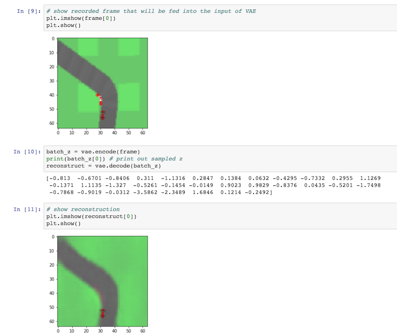
vae_test.ipynb used to examine the VAE trained on CarRacing-v0's extracted data.
In this environment, we use the V and M model as model predictive control (MPC) and train the controller C on the actual environment, rather than inside of the generated environment. So rather than running python train.py you need to run gce_train.bash instead to use the headless X sessions to run the CMA-ES trainer. Because we train in the actual environment, training is slower compared to DoomRNN. By running the training inside a tmux session, you can monitor progress using the plot_training_progress.ipynb notebook by running Jupyter in another tmux session in parallel, which loads the log files being generated.

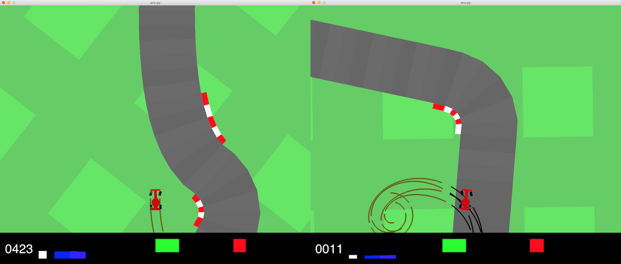
 Training CarRacing-v0 using CMA-ES. Recording C's performance inside of the actual environment.
After 150-200 generations (or around 3 days), it should be enough to get around a mean score of ~ 880, which is pretty close to the required score of 900. If you don’t have a lot of money or credits to burn, I recommend you stop if you are satistifed with a score of 850+ (which is around a day of training). Qualitatively, a score of ~ 850-870 is not that much worse compared to our final agent that achieves 900+, and I don’t want to burn your hard-earned money on cloud credits. To get 900+ it might take weeks (who said getting SOTA was easy? :). The final models are saved in log/*.json and you can test and view them the usual way.
Contributing
There are many cool ideas to try out – For instance, iterative training methods, transfer learning, intrinsic motivation, other environments.
If you want to extend the code and try out new things, I recommend modifying the code and trying it out to solve a specific new environment, and not try to improve the code to work for multiple environments at the same time. I find that for research work, and when trying to solve difficult environments, specific custom modifications are usually required. You are welcome to submit a pull request with a self-contained subdirectory that is tailored for a specific challenging environment that you had attempted to solve, with instructions in a README.md file in your subdirectory.
Citation
If you found this code useful in an academic setting, please cite:
@incollection{ha2018worldmodels,

  title = {Recurrent World Models Facilitate Policy Evolution},

  author = {Ha, David and Schmidhuber, J{\"u}rgen},

  booktitle = {Advances in Neural Information Processing Systems 31},

  pages = {2451--2463},

  year = {2018},

  publisher = {Curran Associates, Inc.},

  url = {https://papers.nips.cc/paper/7512-recurrent-world-models-facilitate-policy-evolution},

  note = "\url{https://worldmodels.github.io}",

}