In a previous post, we’ve looked at a generative algorithm that can produce images of digits at arbitrary high resolutions, while training on on a set of low resolution images, such as MNIST or CIFAR-10. This post explores several changes to the previous model to produce more interesting results.

Specifically, we removed the use of pixel-by-pixel reconstruction loss in the Variation Autoencoder. The discriminator network used to detect fake images is replaced by a classifier network. The generator network used previously had been a relatively large network consisting of 4 layers of 128 fully connected nodes, and we explore replacing this network with a much deeper network of 96 layers, but only with only 6 nodes in each layer. Finally, we explore initialising parts of the weights to be relatively much larger than normal neural network weight initialisation methods, for the purpose of producing art, and also discuss the benefits of under-training the network.

Motivation

Until recently, much of machine learning research has been about testing a model against certain quantitative metrics and benchmarks. Metrics are quite clear in certain machine learning tasks, such as classification accuracy, prediction error, or the score obtained from playing an ATARI game.

Researchers working on generative algorithms also needed to devise a set of quantitative scores to evaluate how well the algorithm performed. When an English sentence is translated to Chinese, the generated sentence is usually compared against a test dataset using likelihood loss, or some human-engineered metric like BLEU scores. Same goes for the generation of text data, music, or images.

While I think metrics are useful to measure performance of machine learning algorithms, we must be more careful when using them on things that are less measurable. For instance, I believe that once machine learning algorithms are used to create something that is supposed to be artistic, we should think more carefully about how we define the metrics to score our algorithms. When the machine is training your art-generating model, what exactly is it optimising for?

Which ones would you hang in your living room?

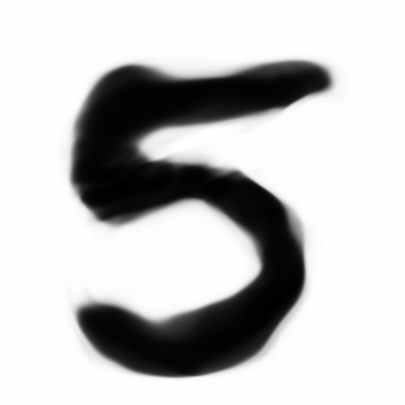
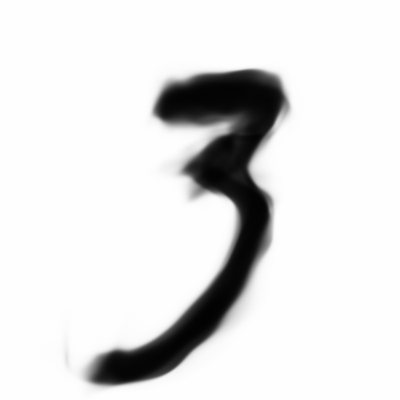
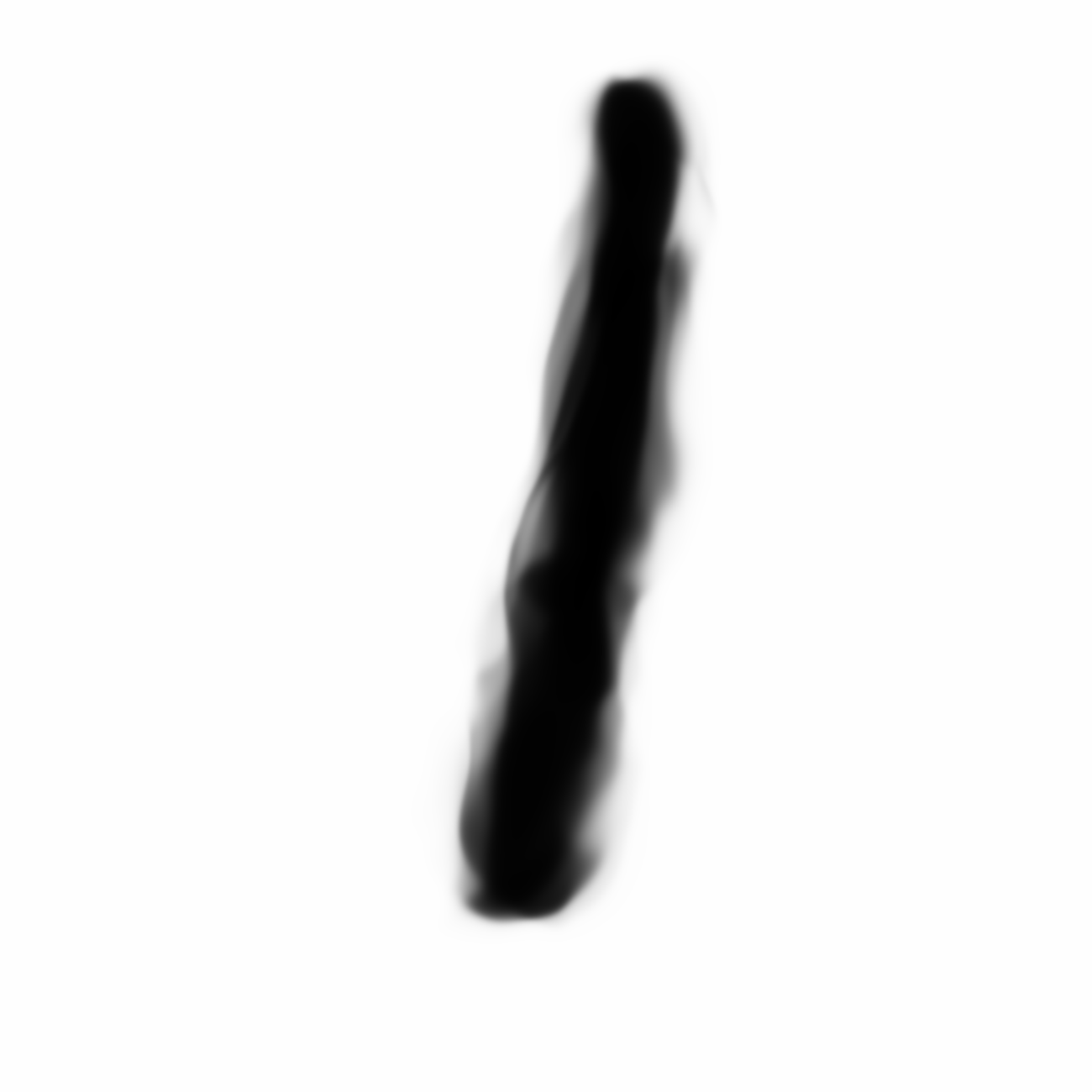
Below are sample images of digits drawn from previous blog post’s generative network. Random gaussian latent vectors were generated from numpy.random and fed into the generative network to obtain these images.

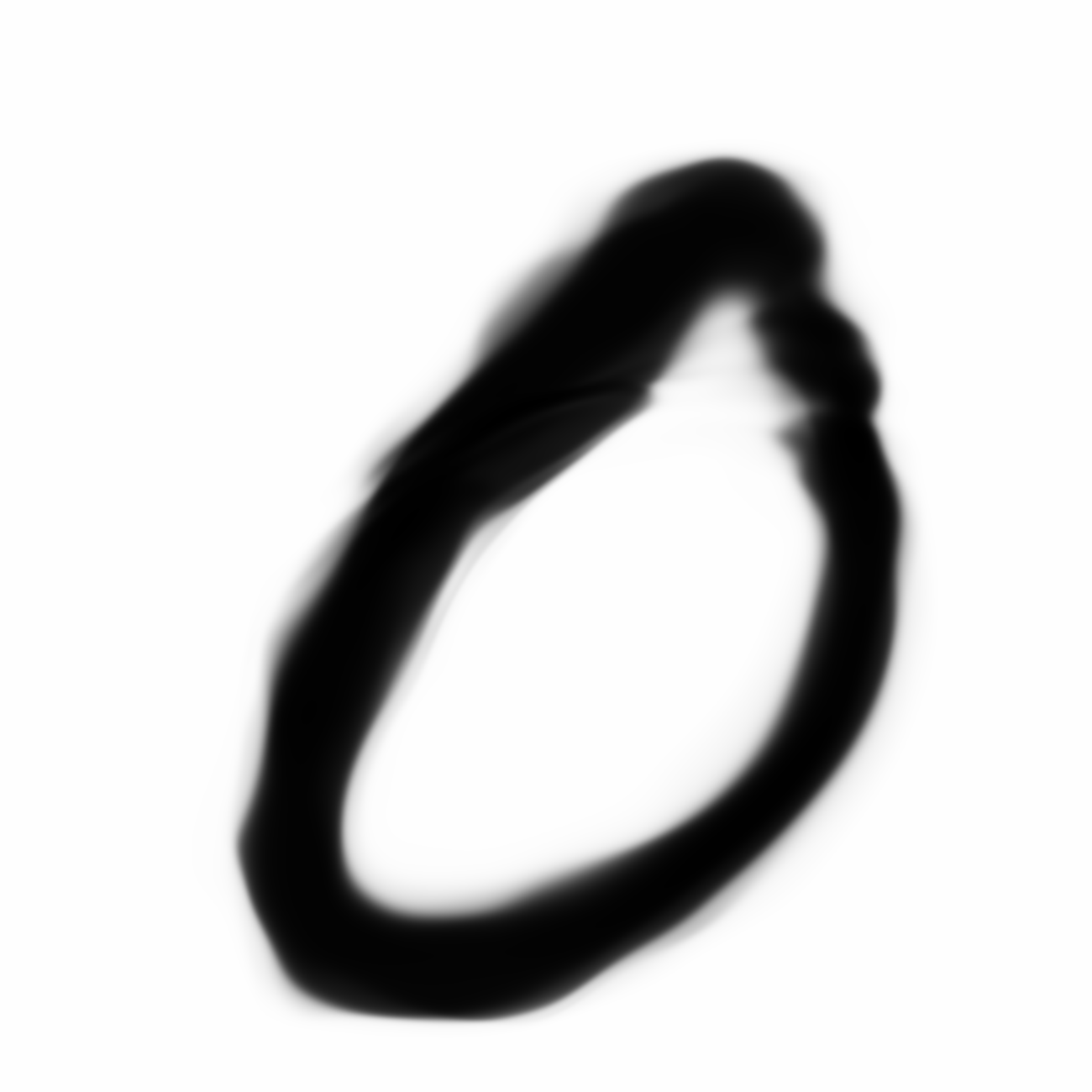
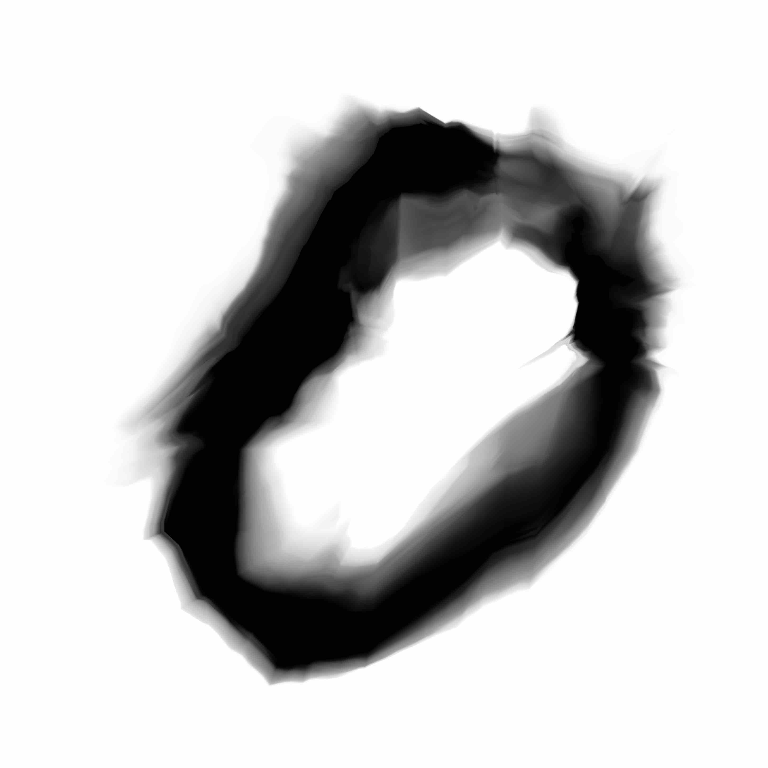
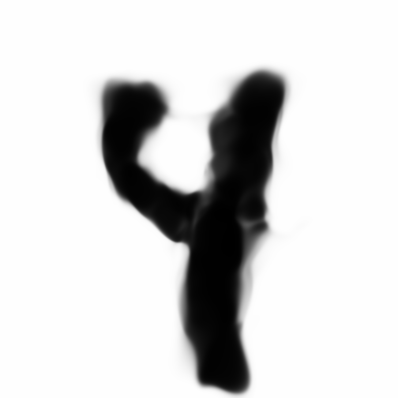
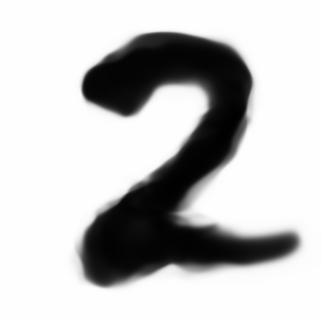
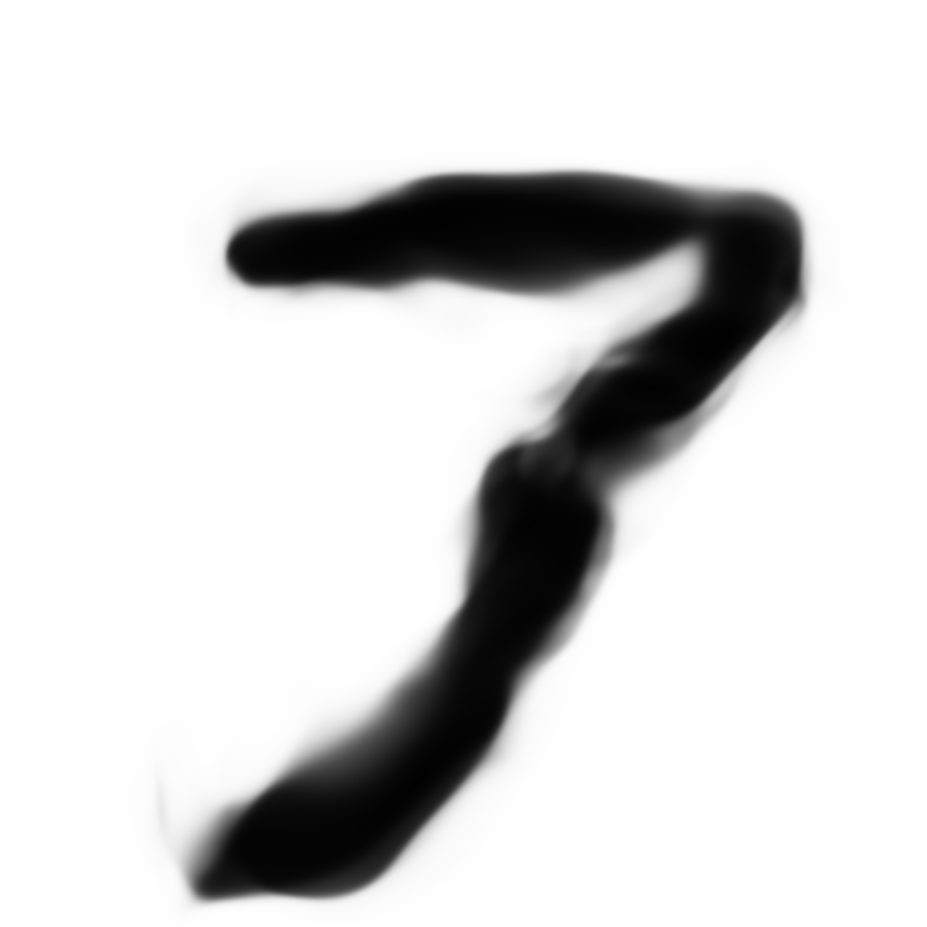
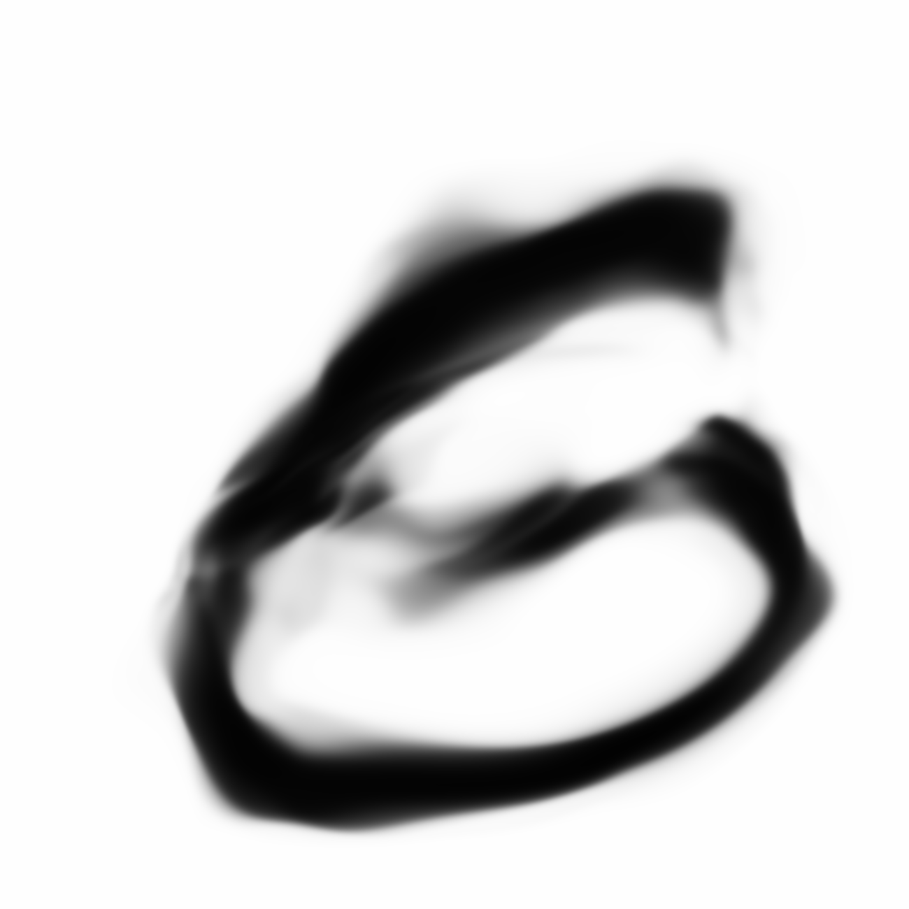
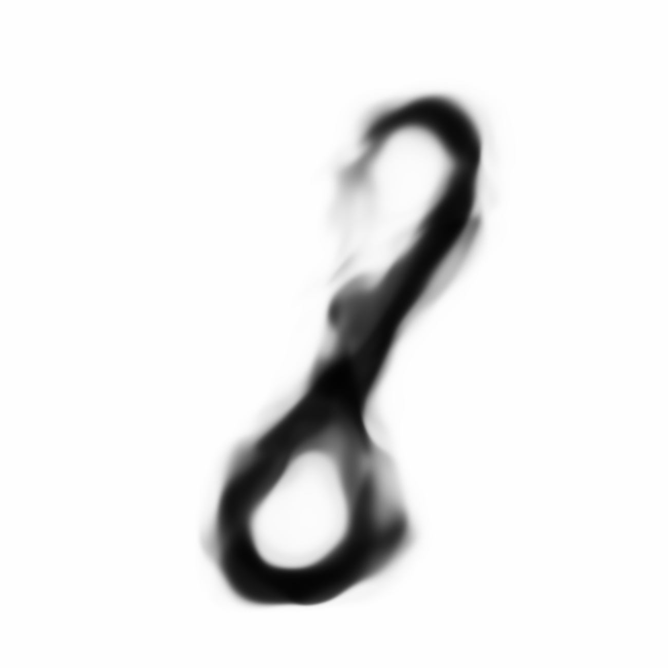
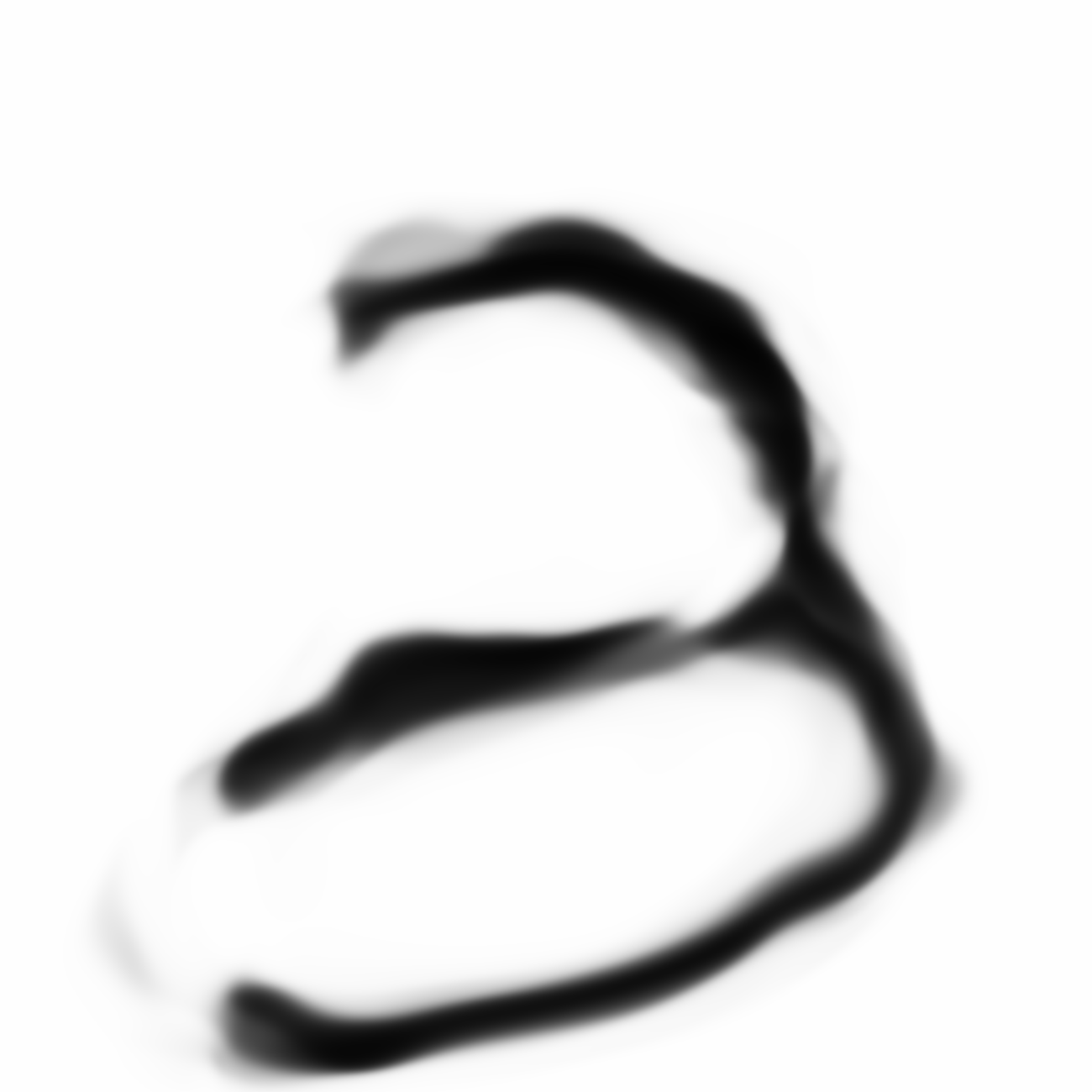
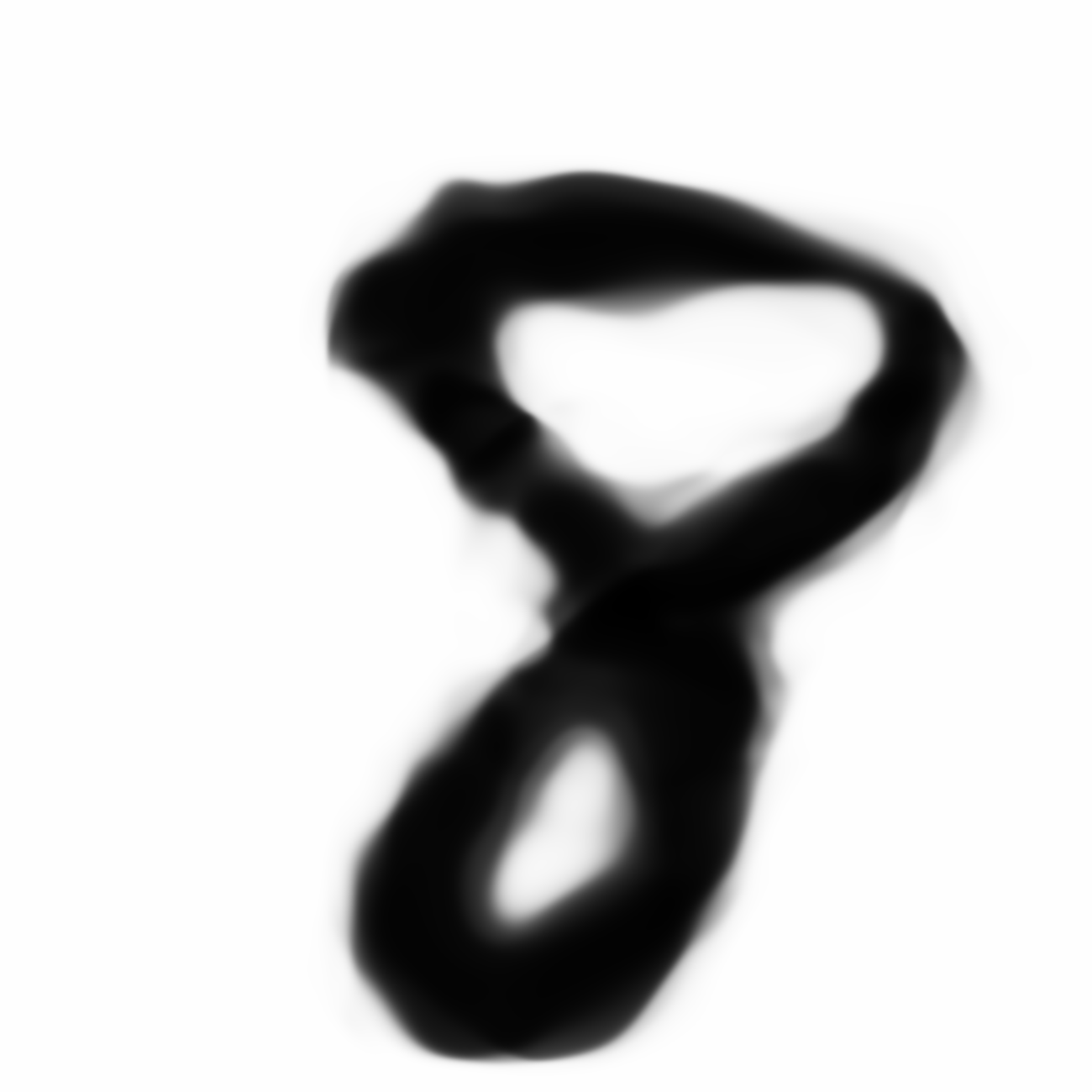
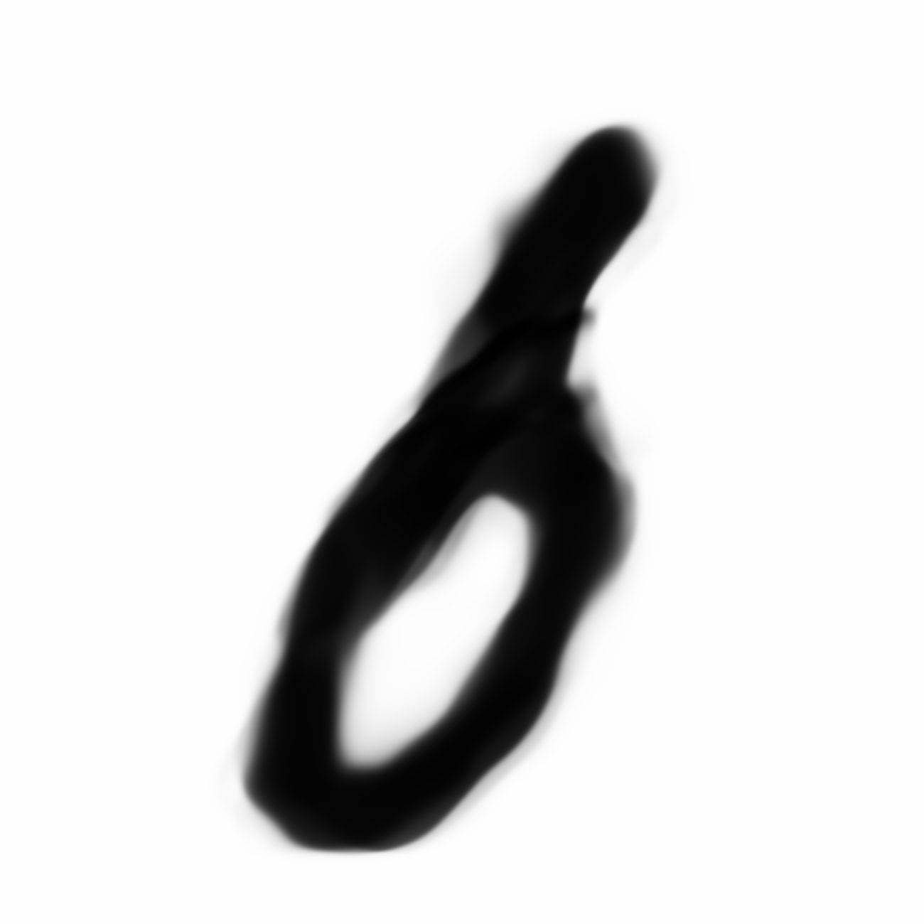
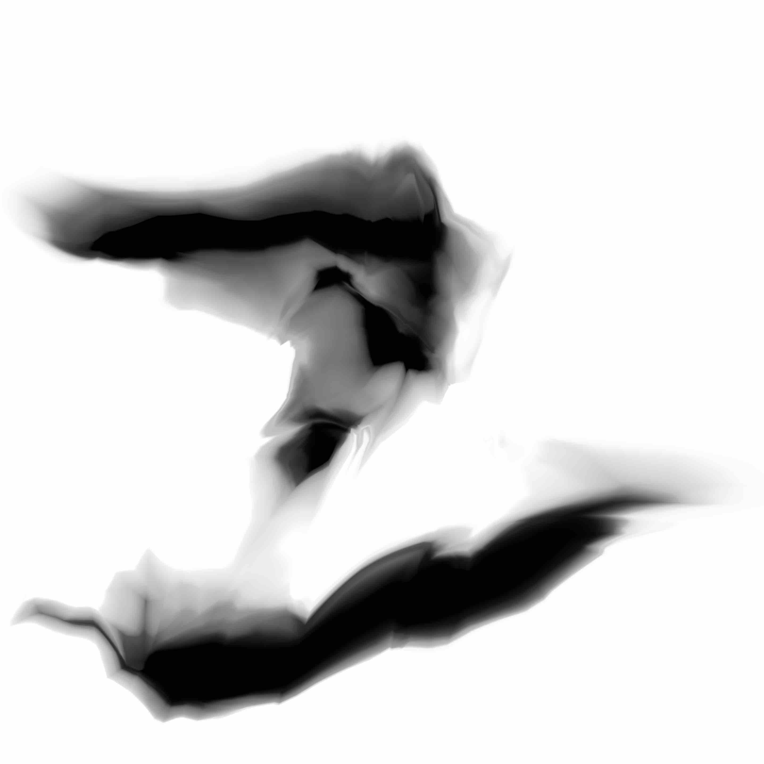
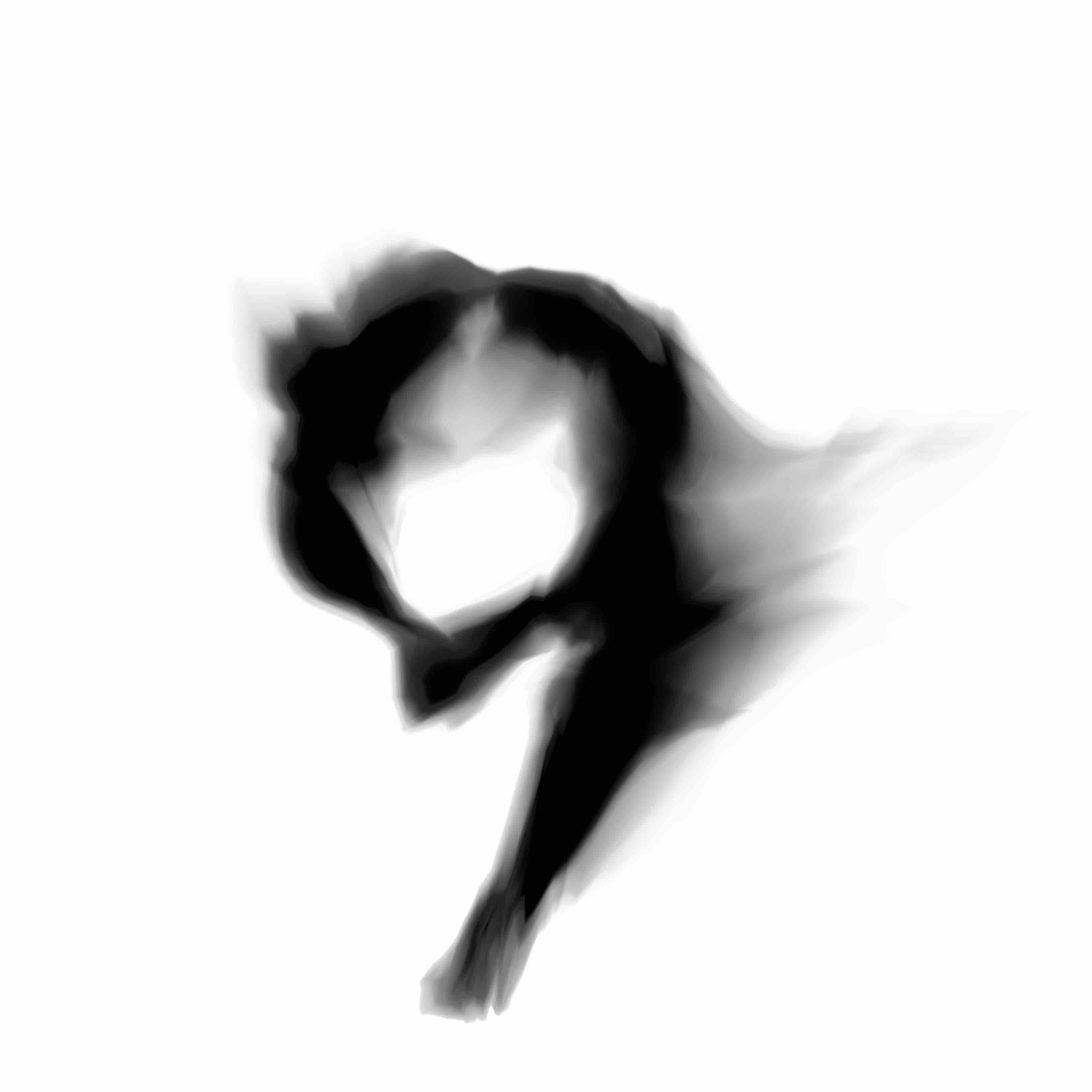
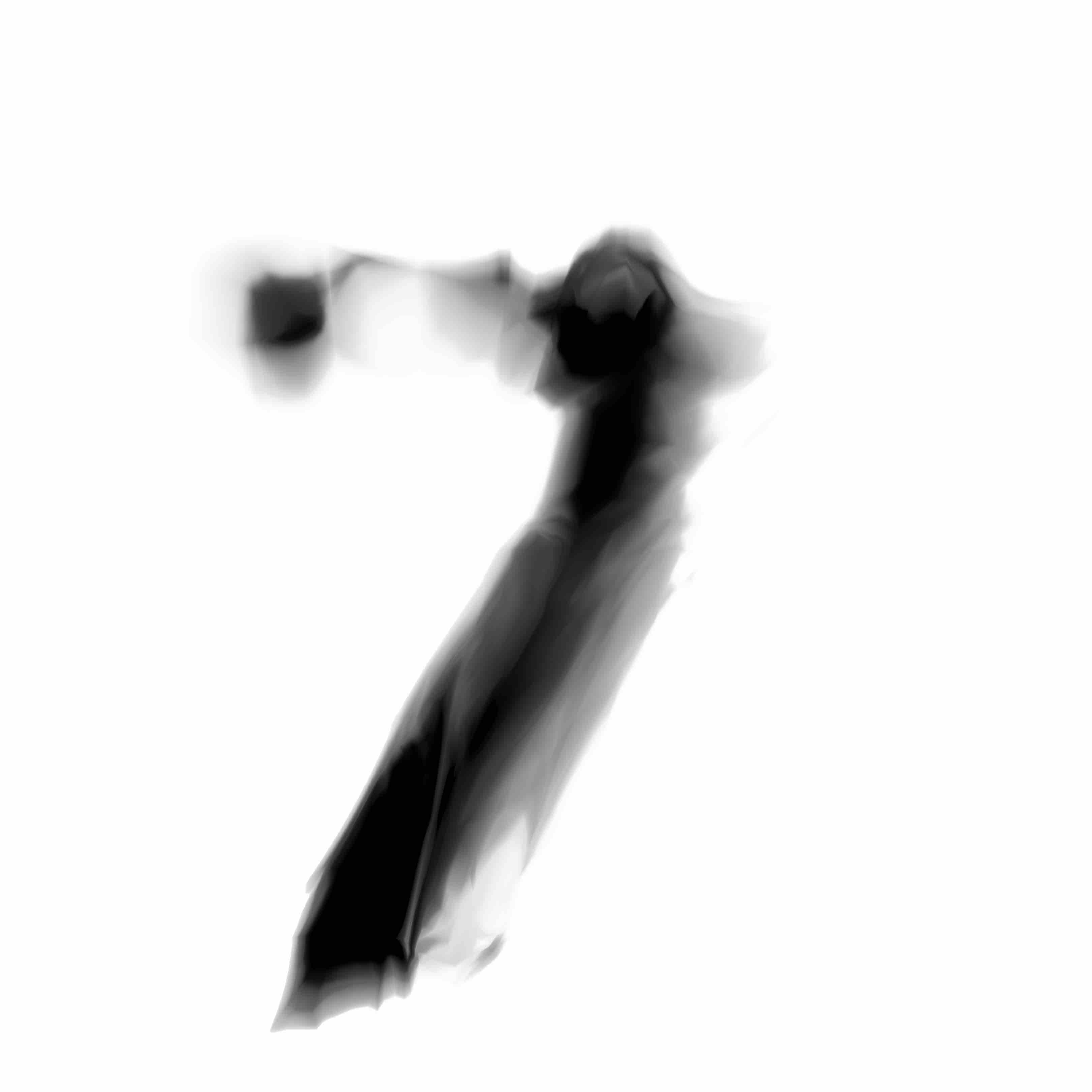
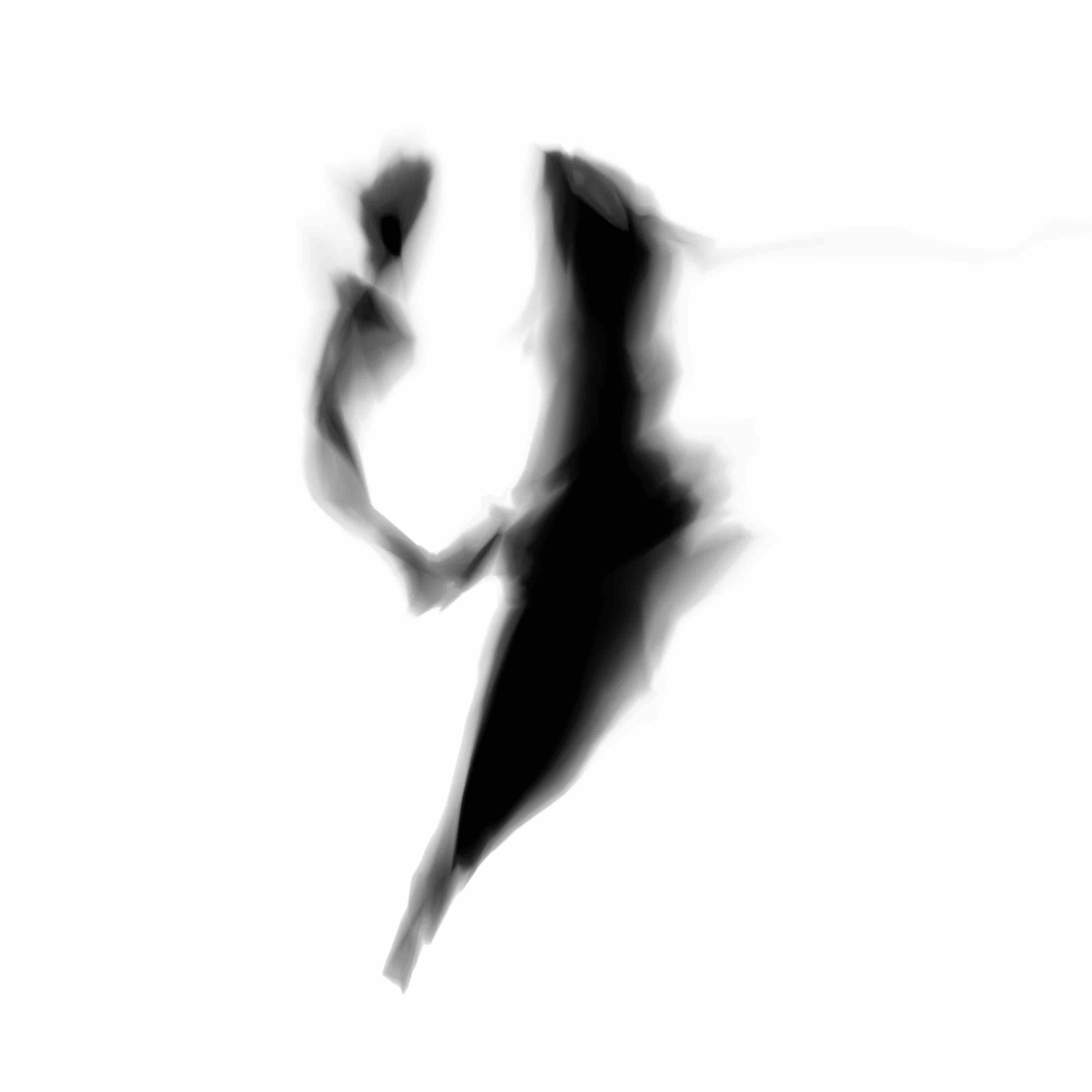
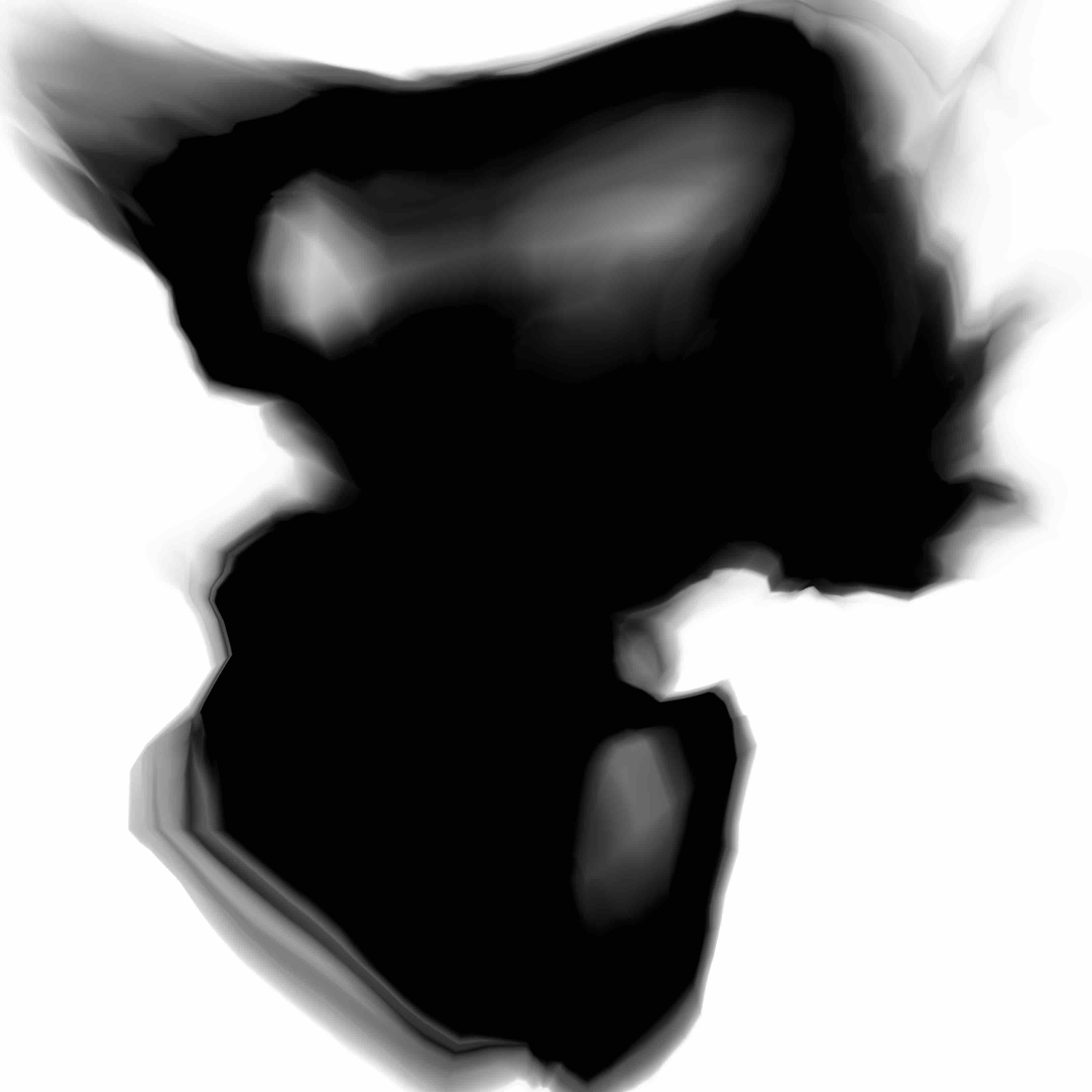
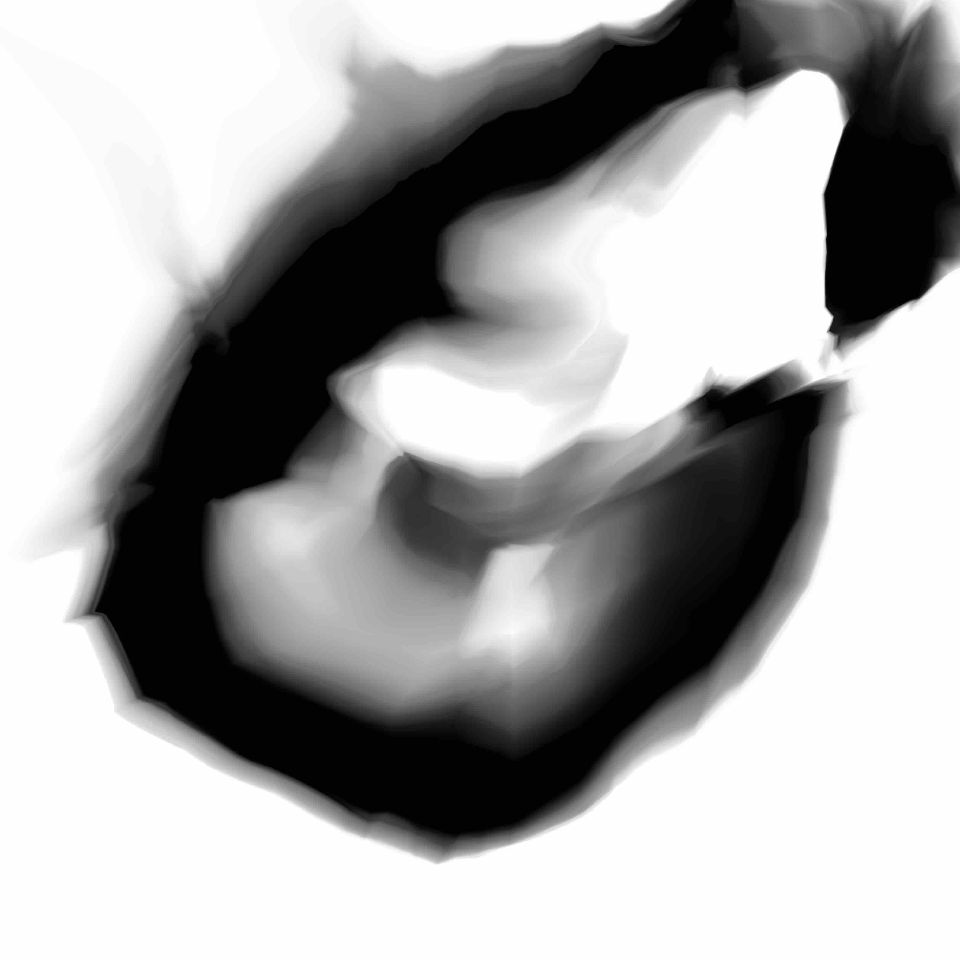
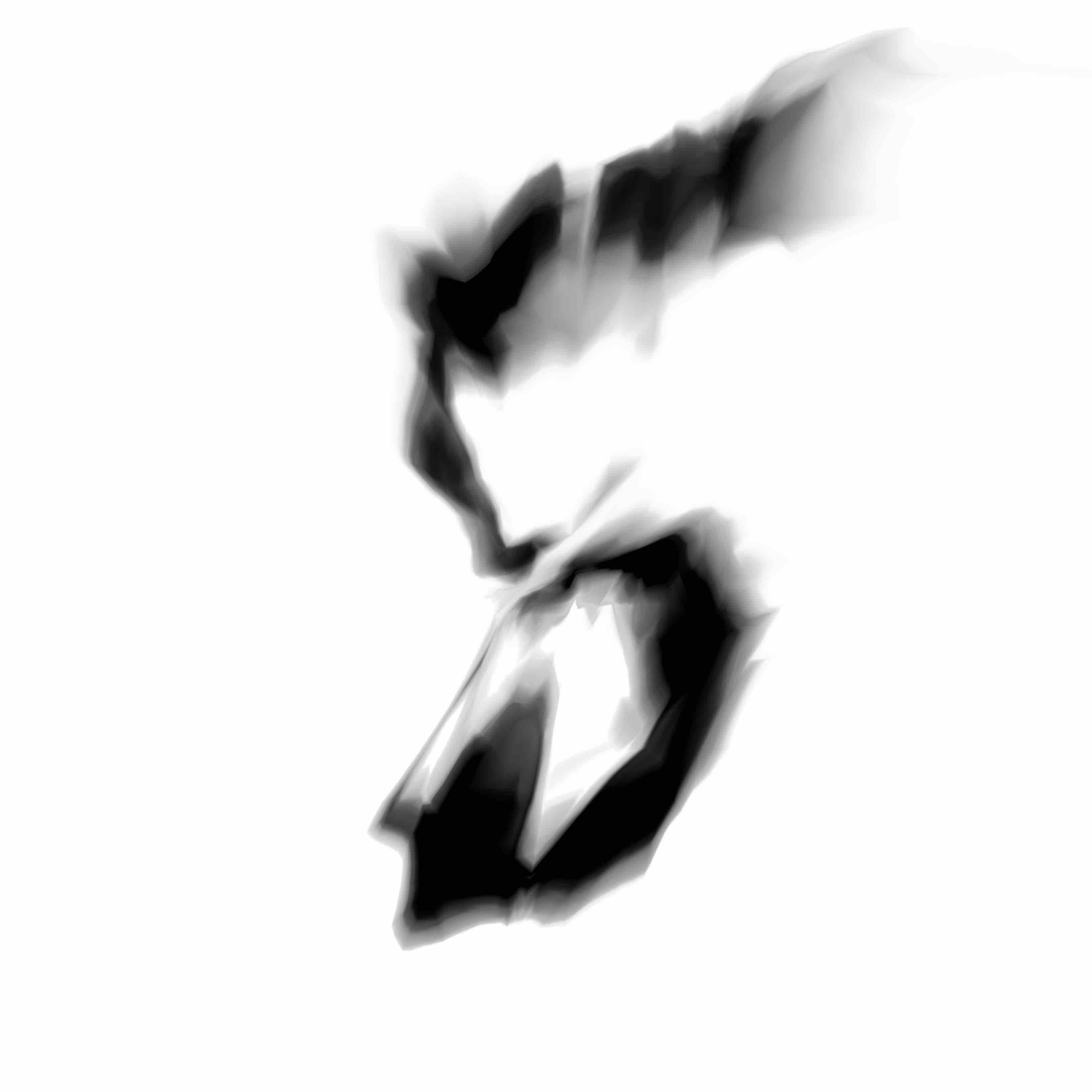
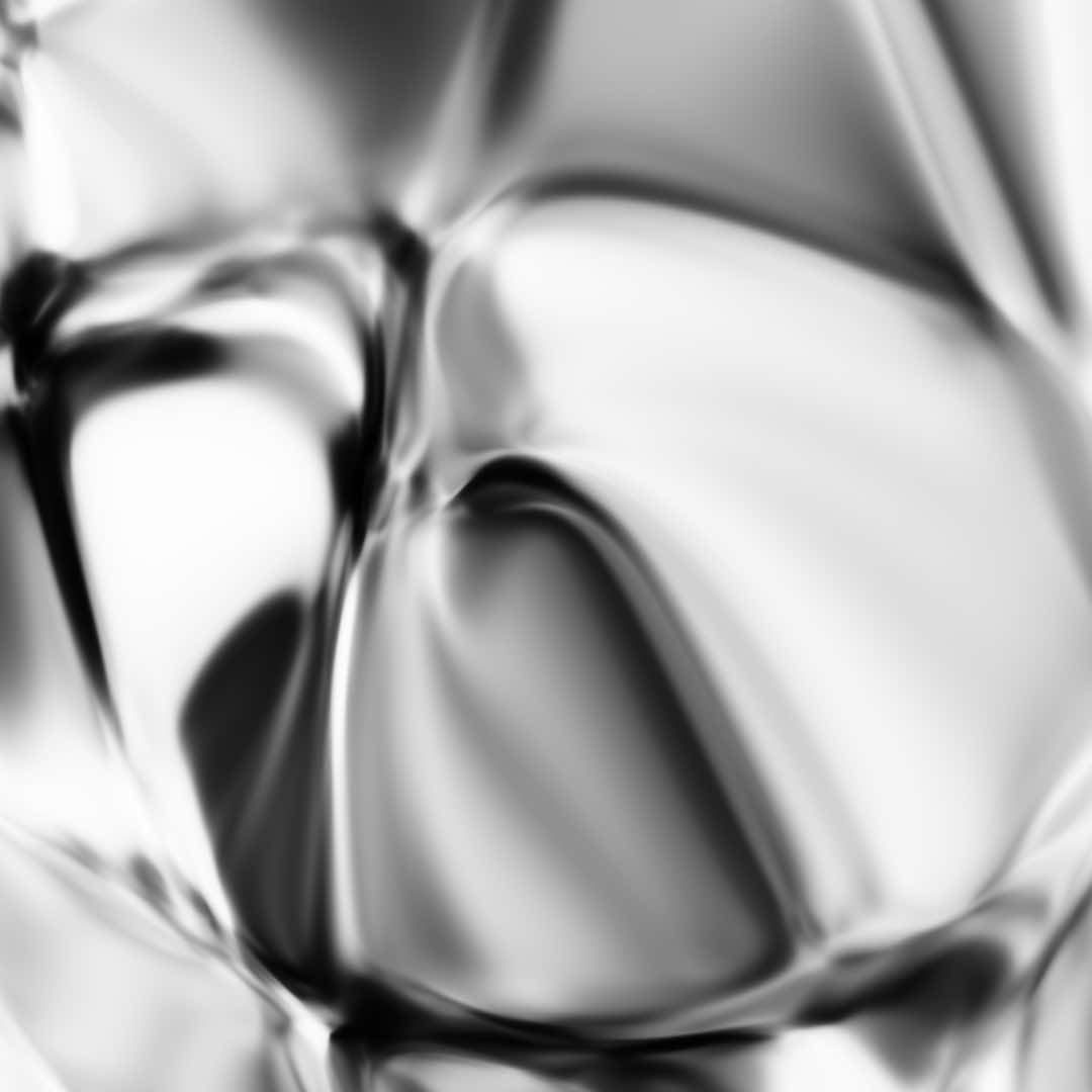
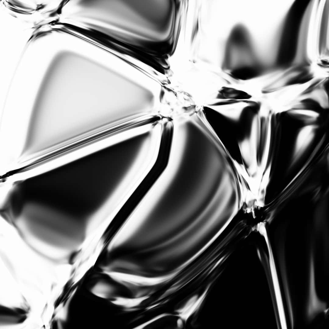
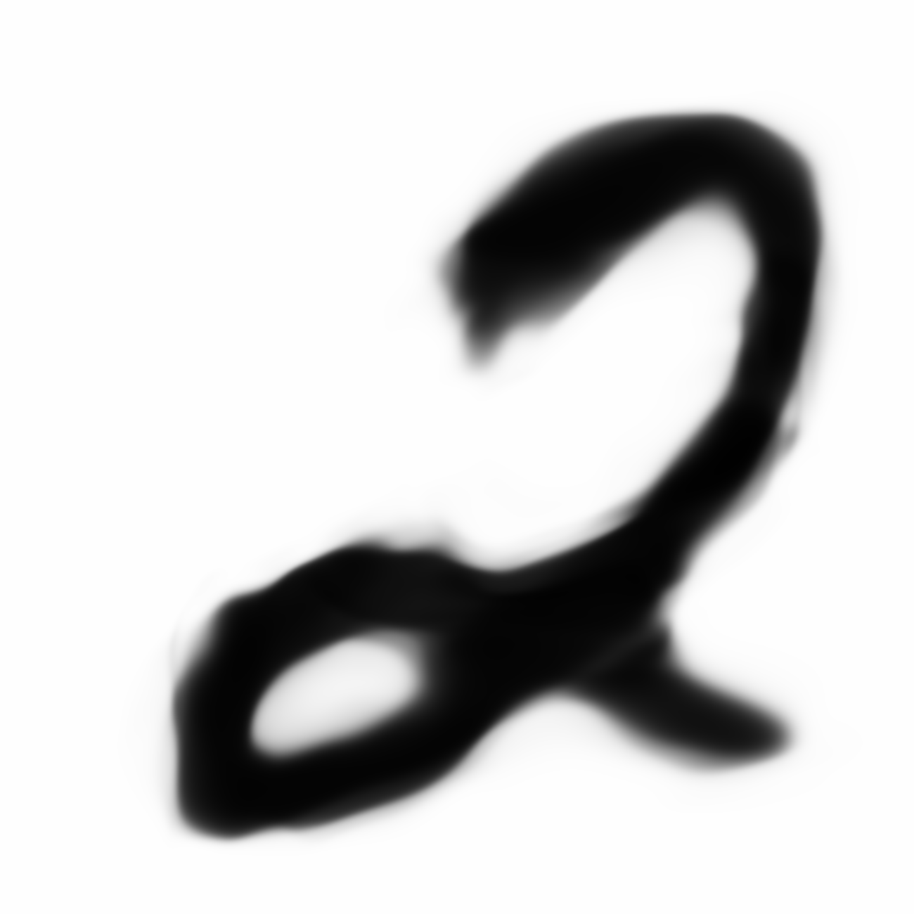
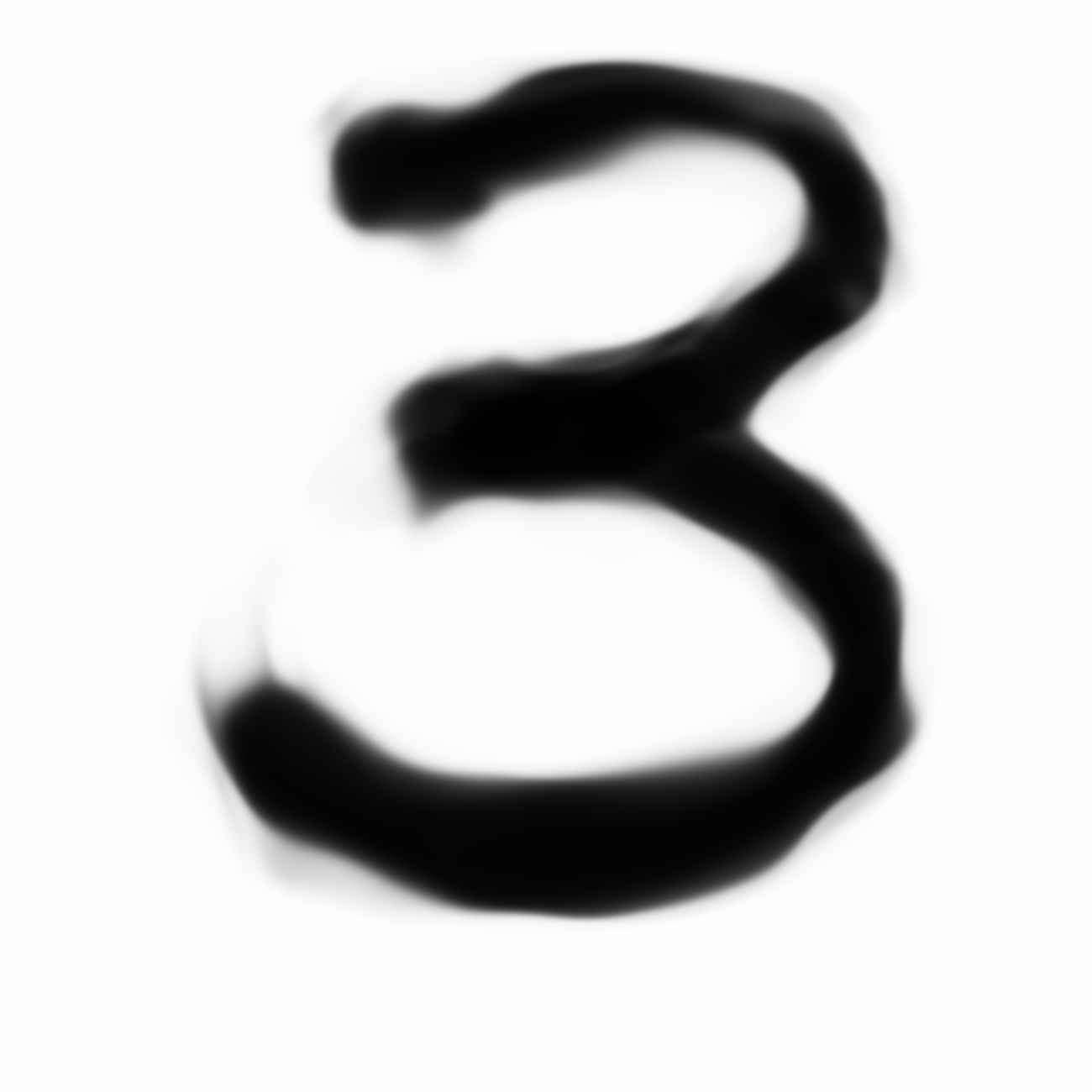
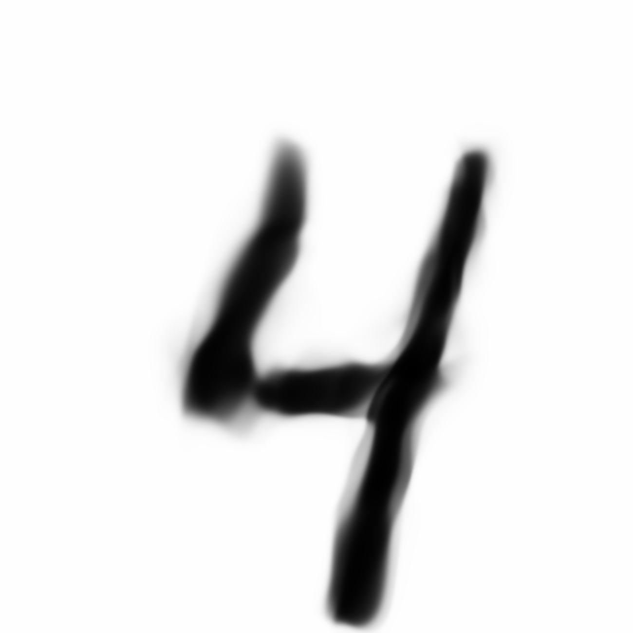
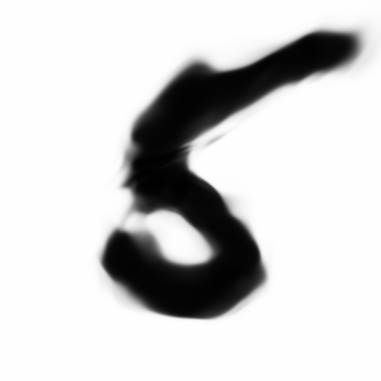
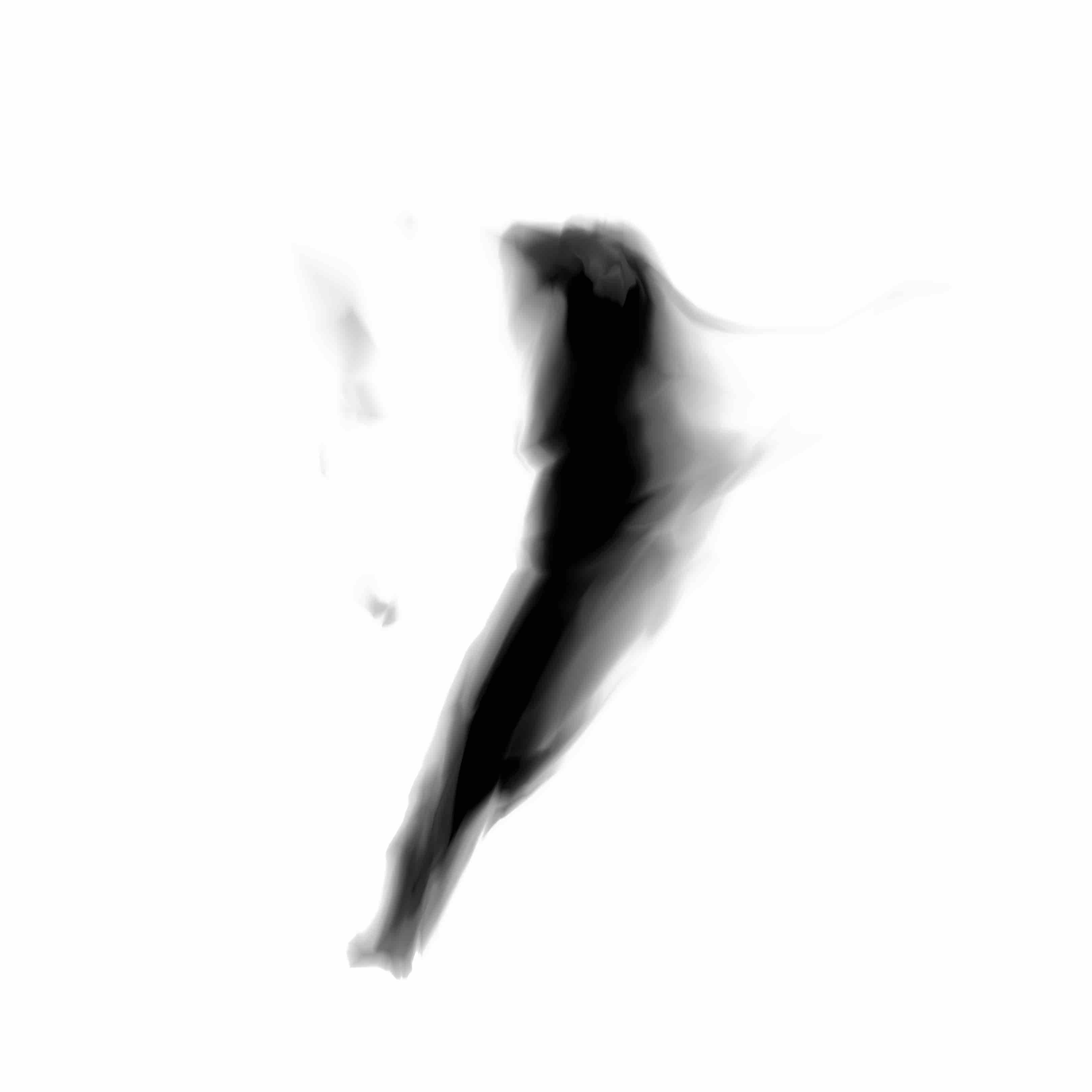
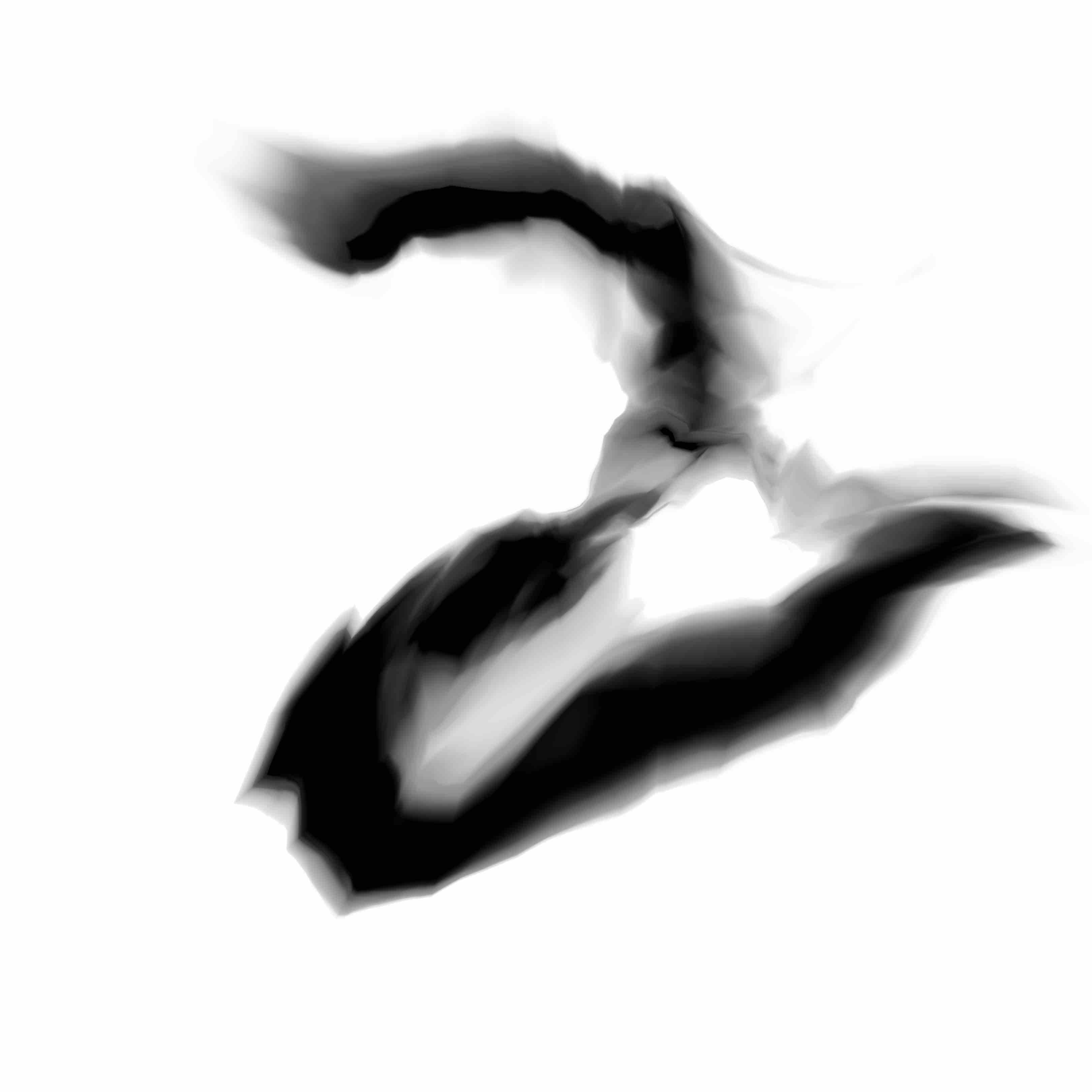
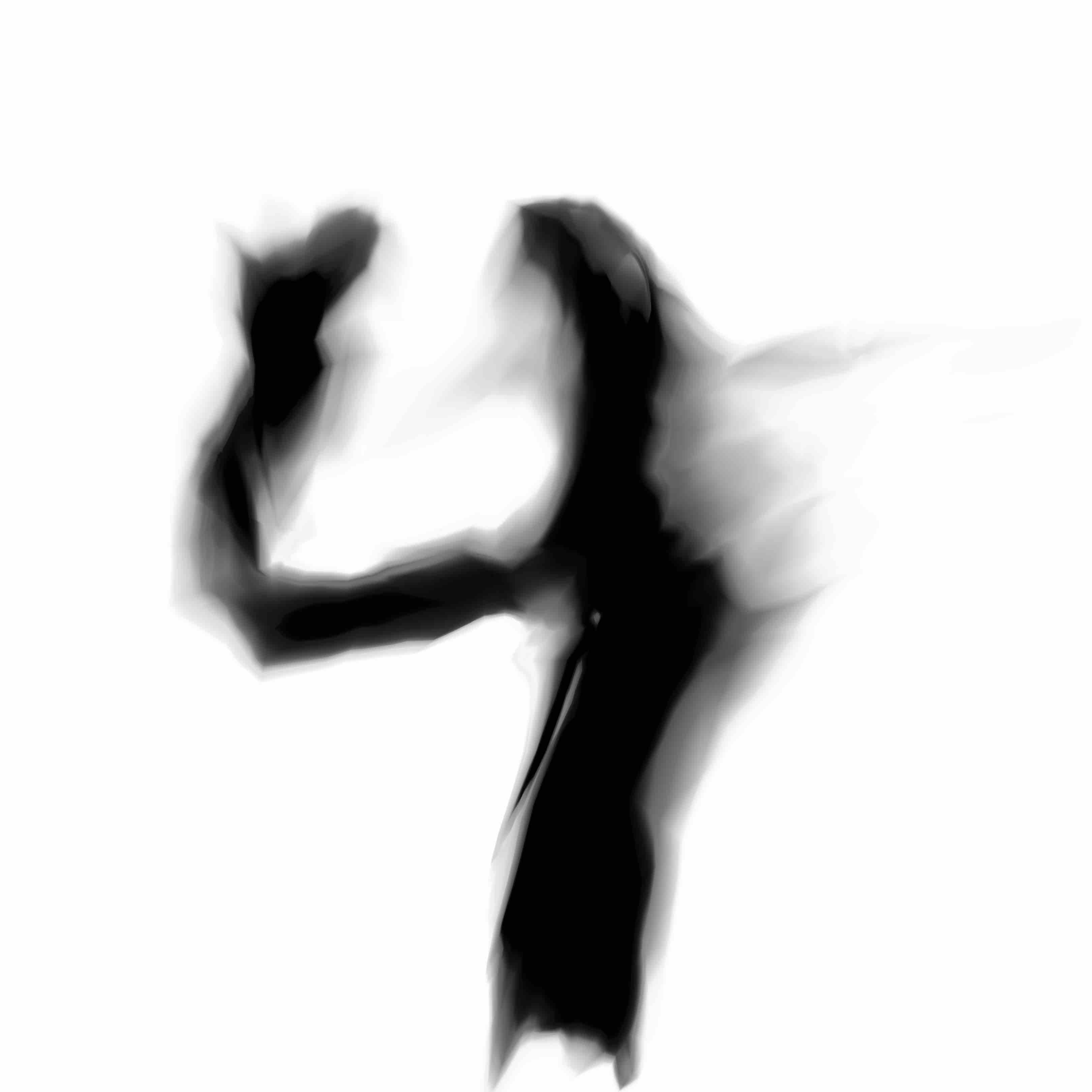
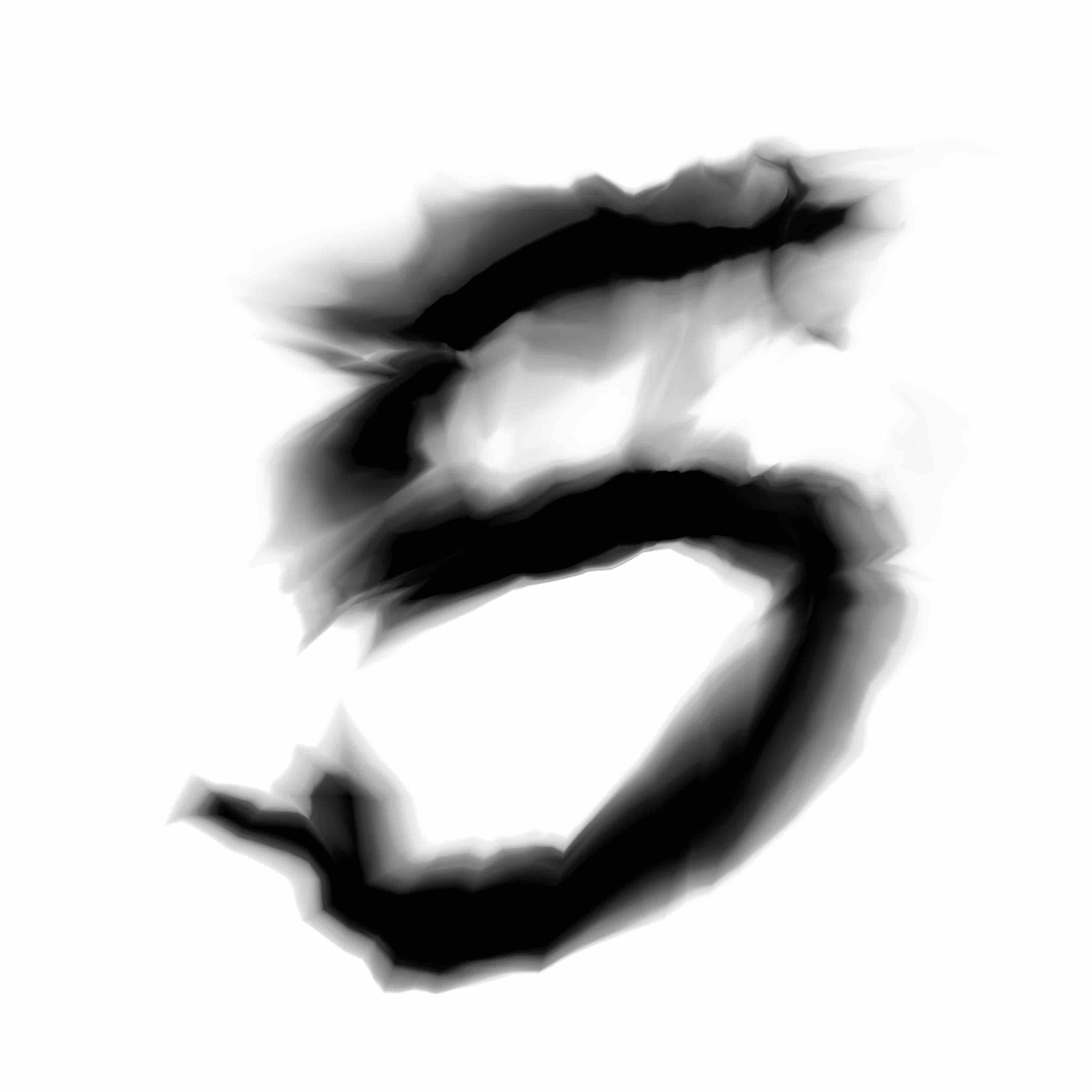
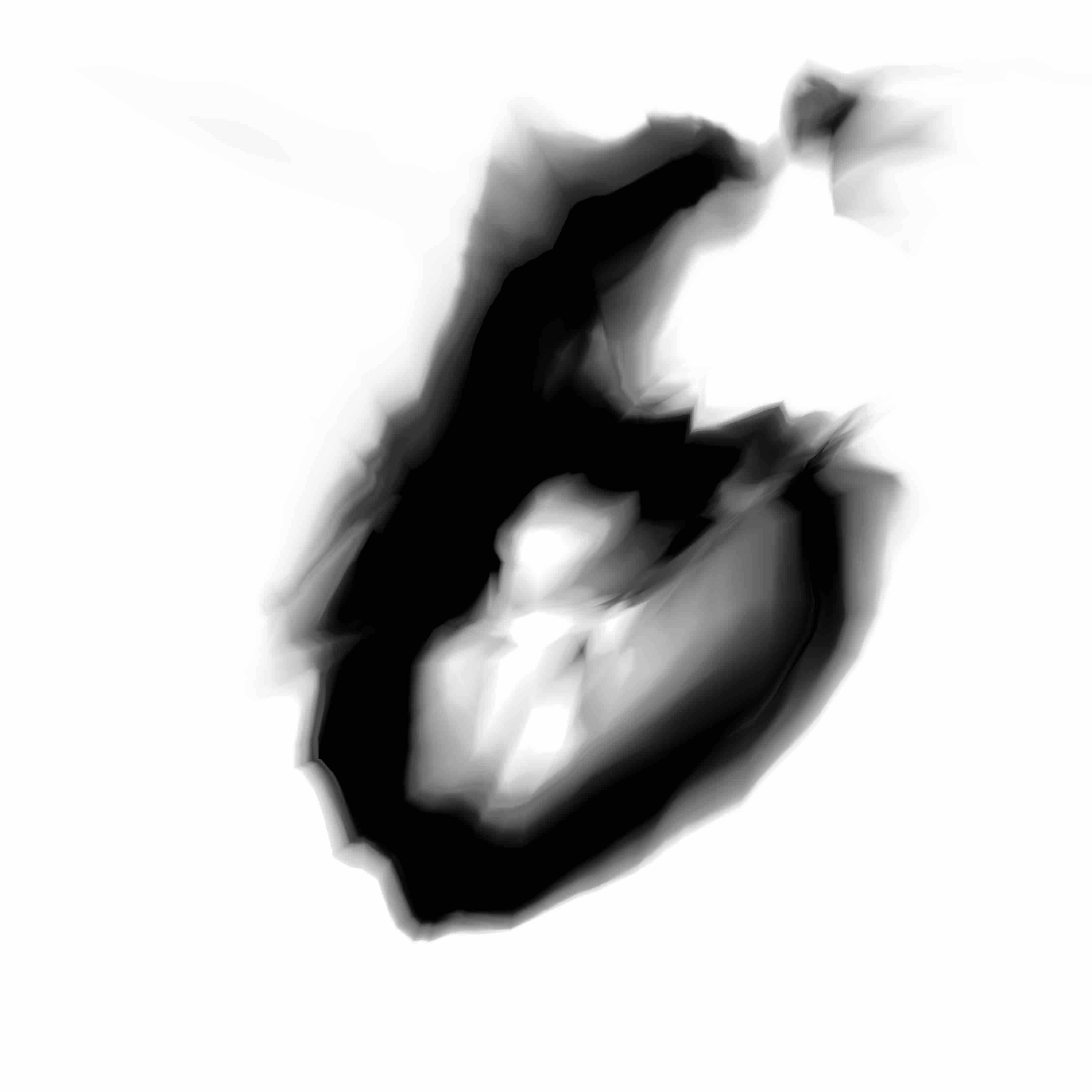
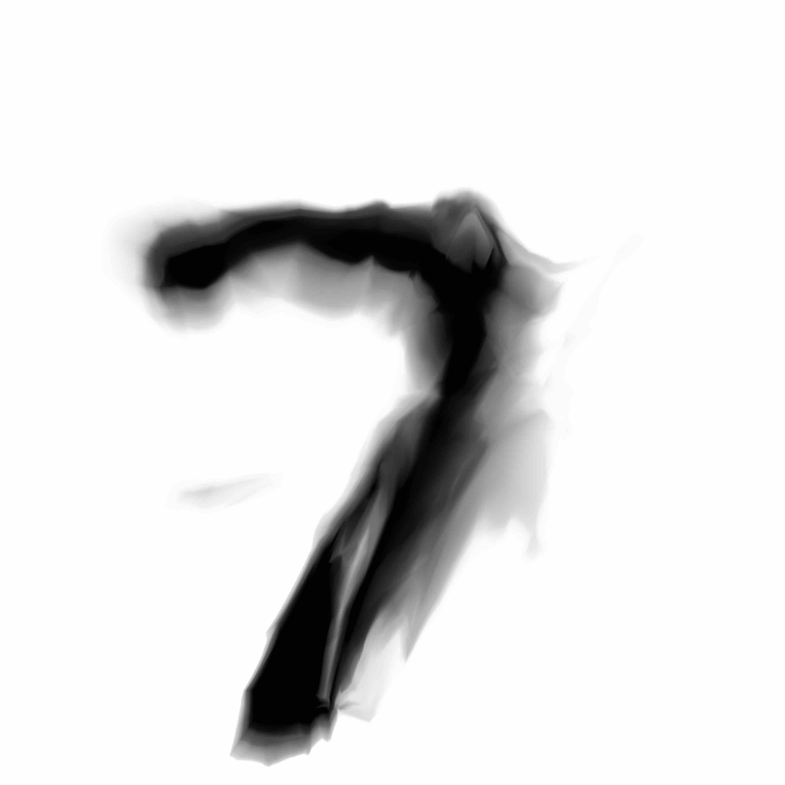
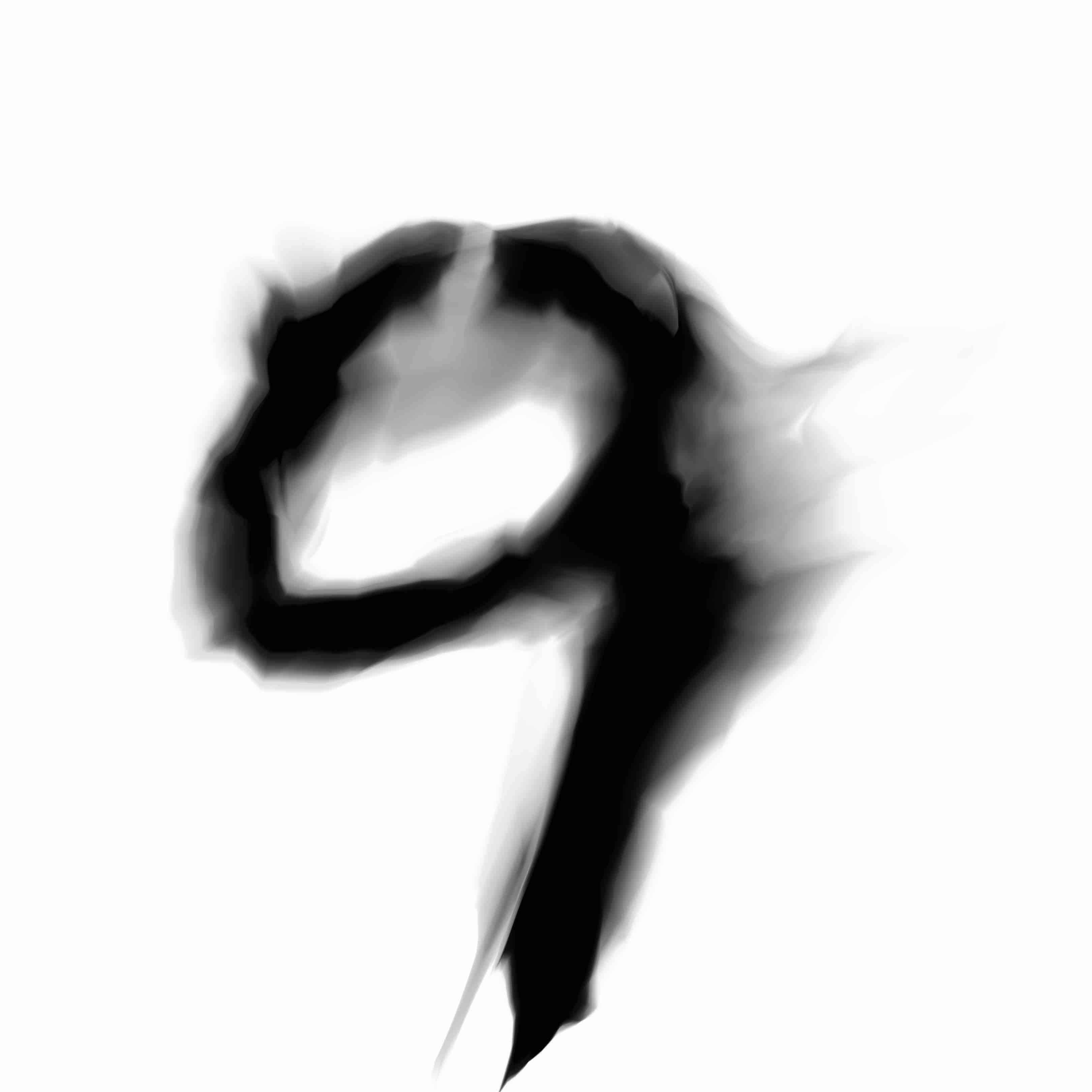
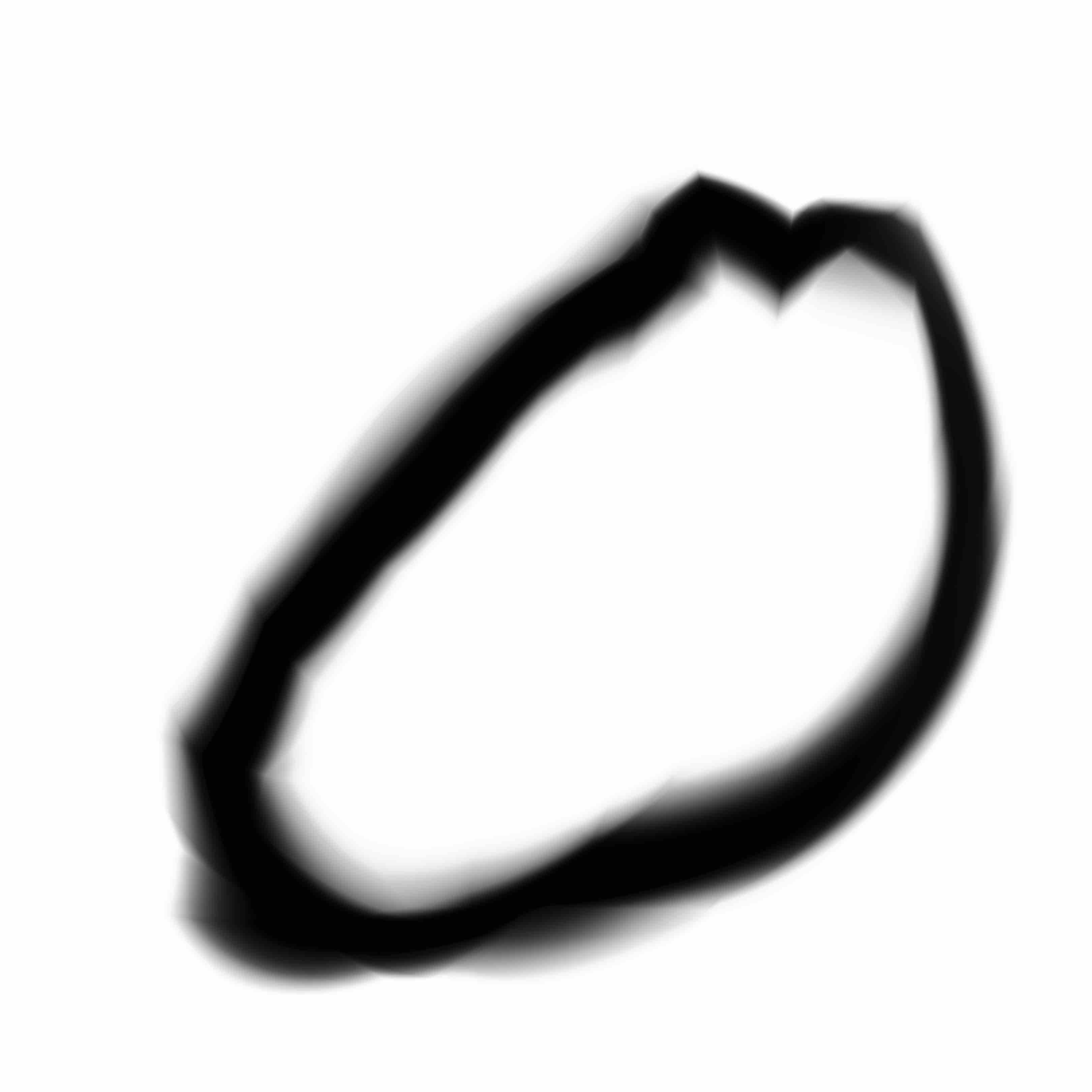
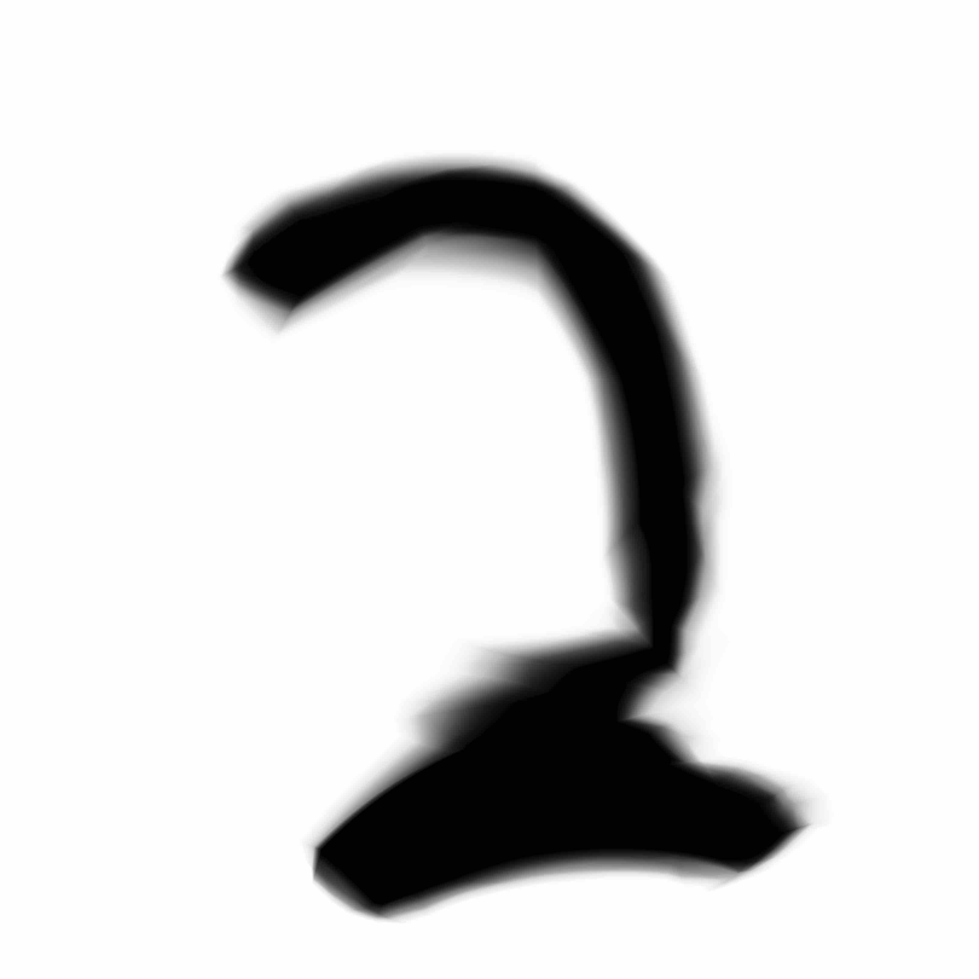
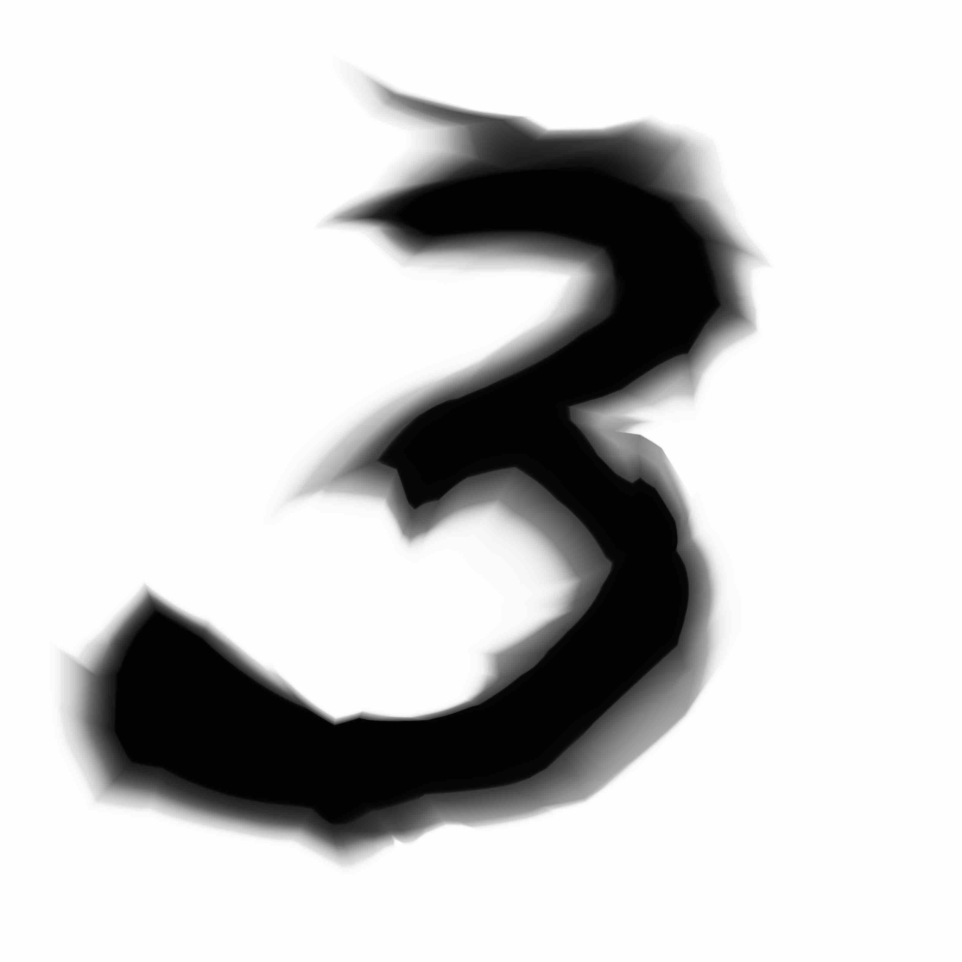
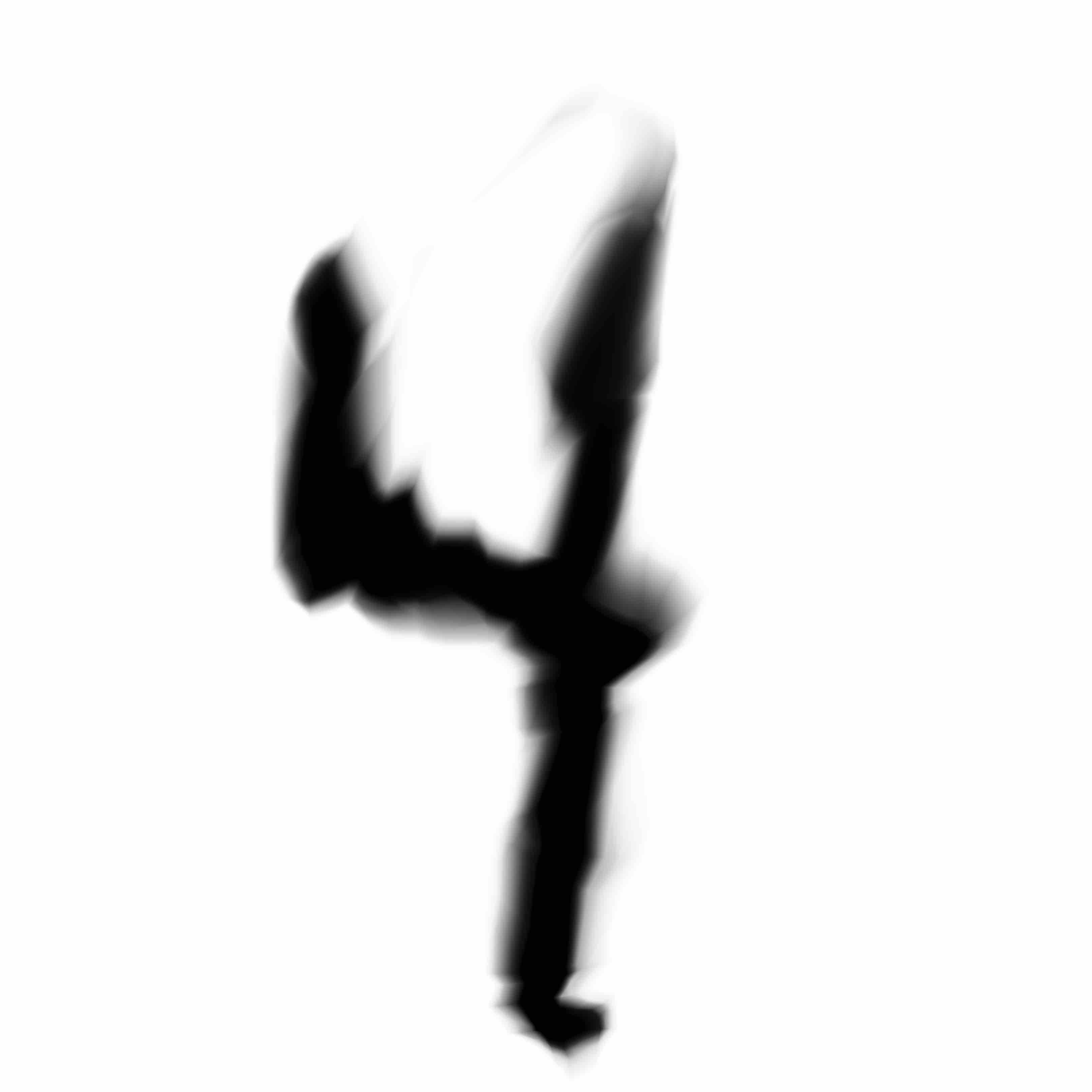
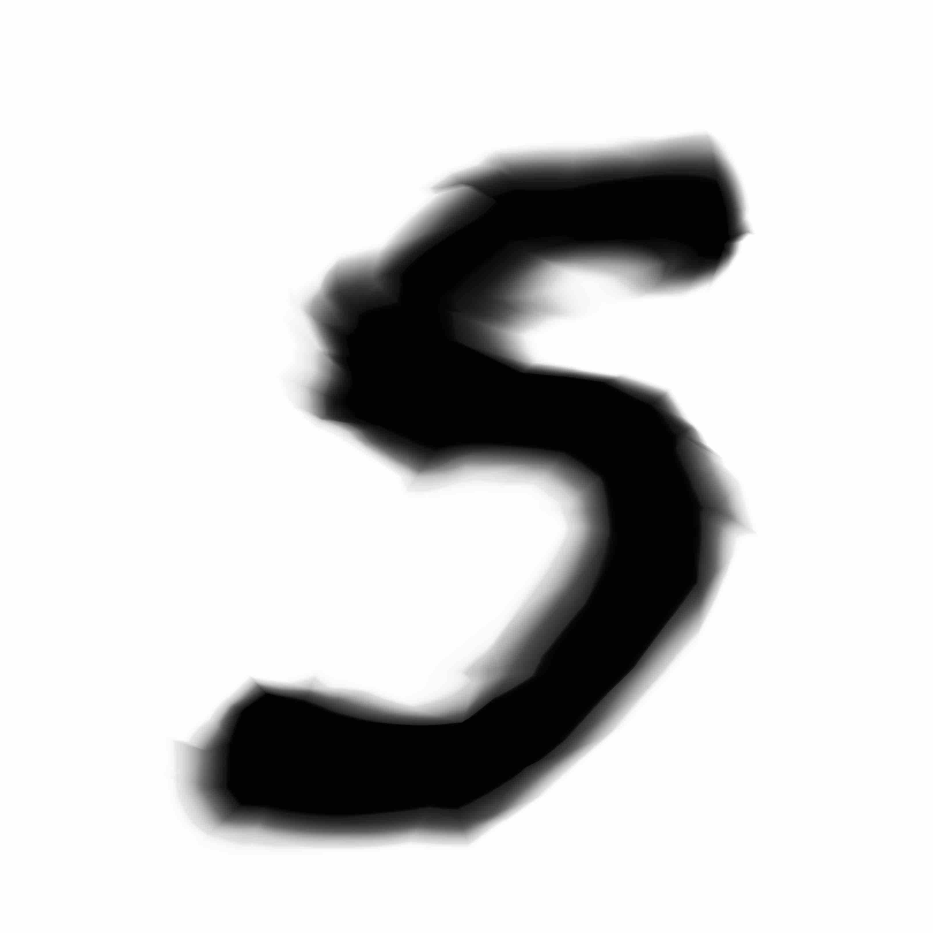
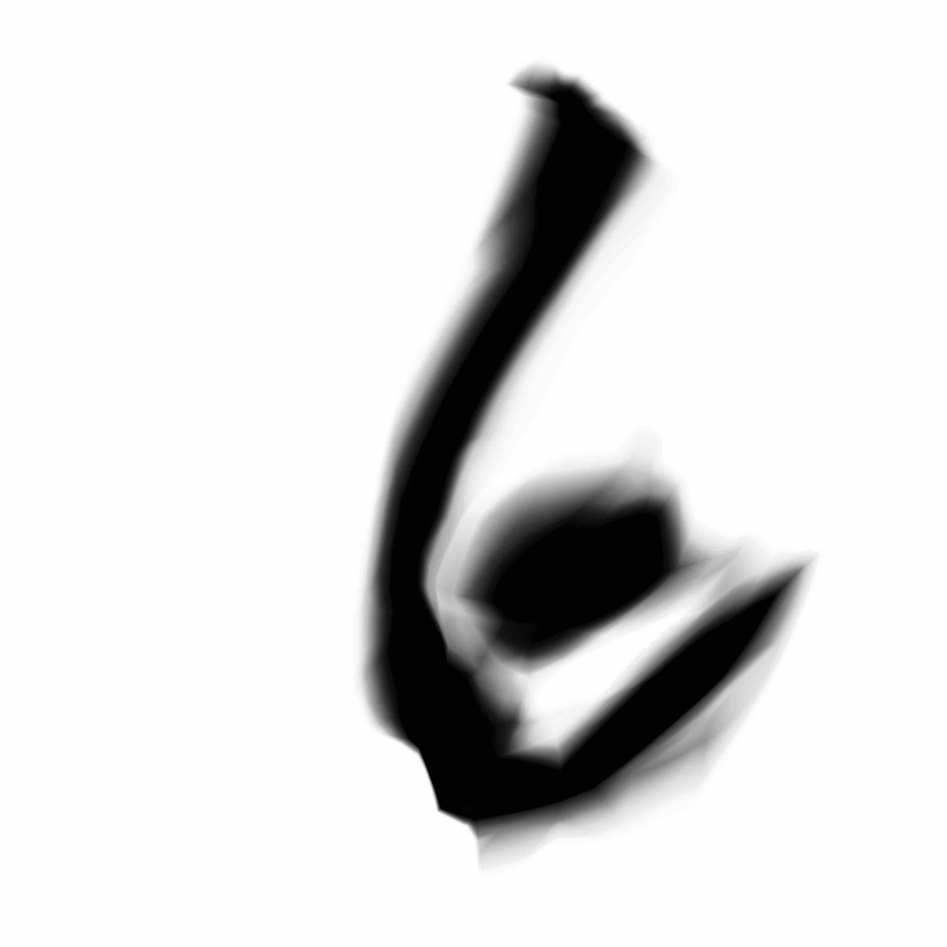
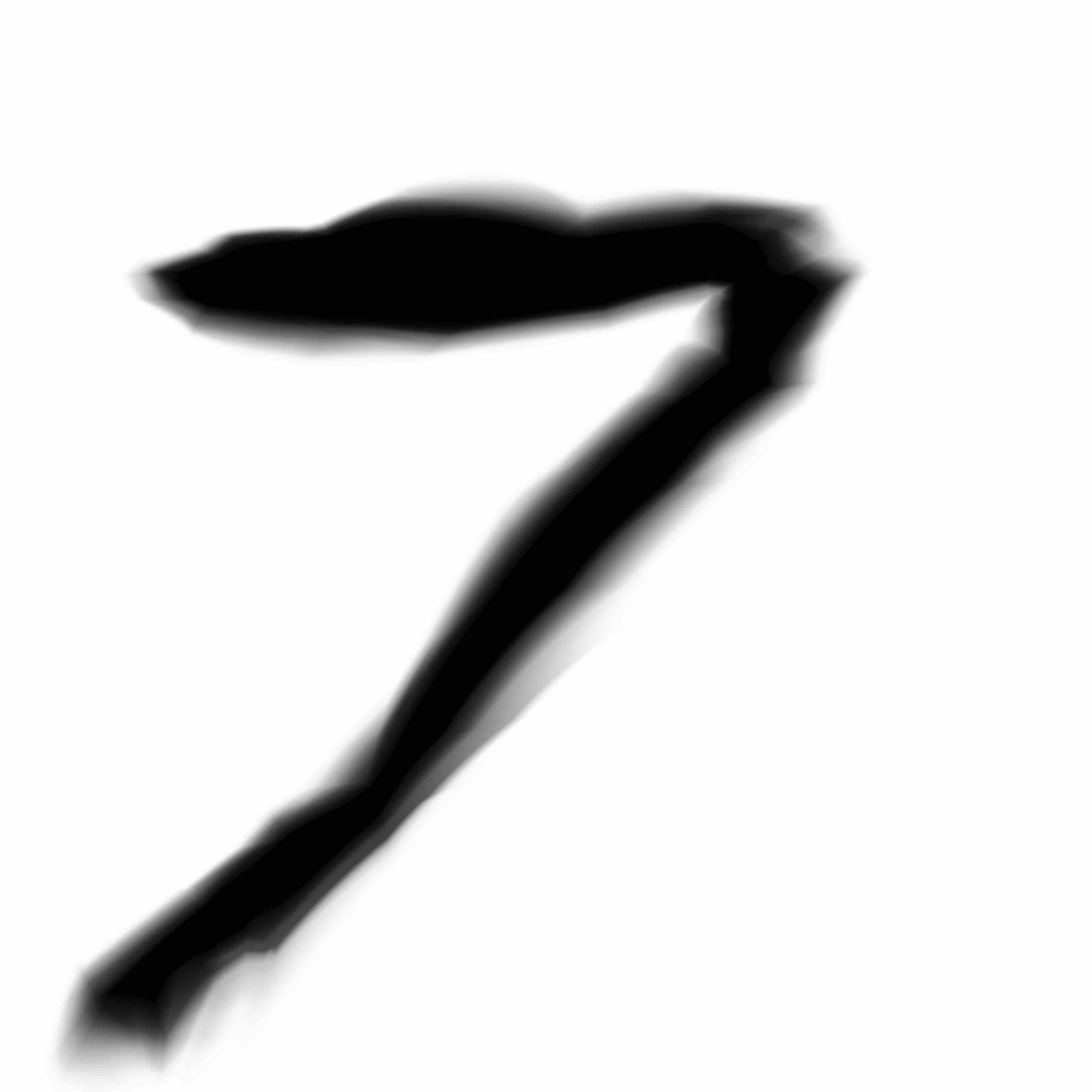
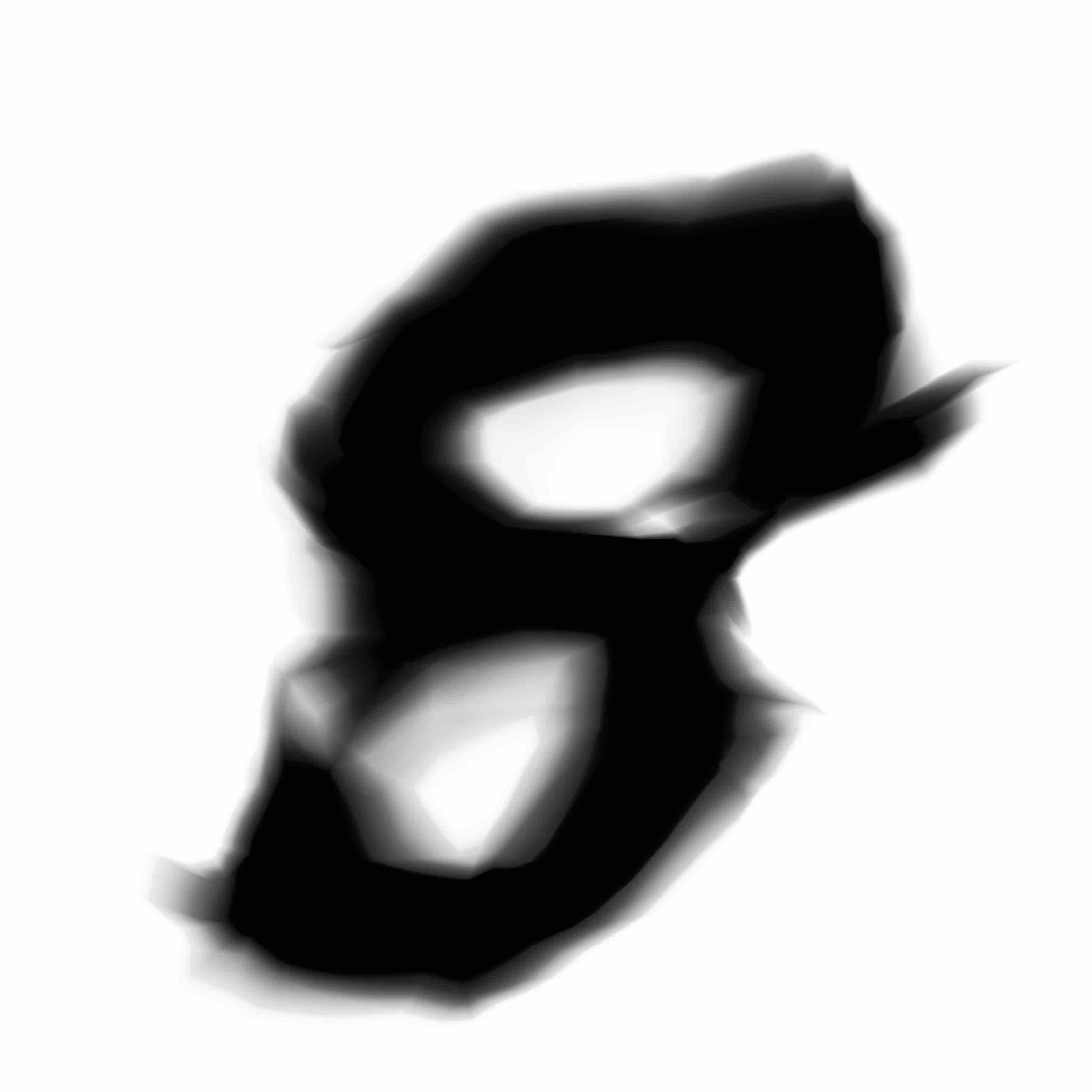
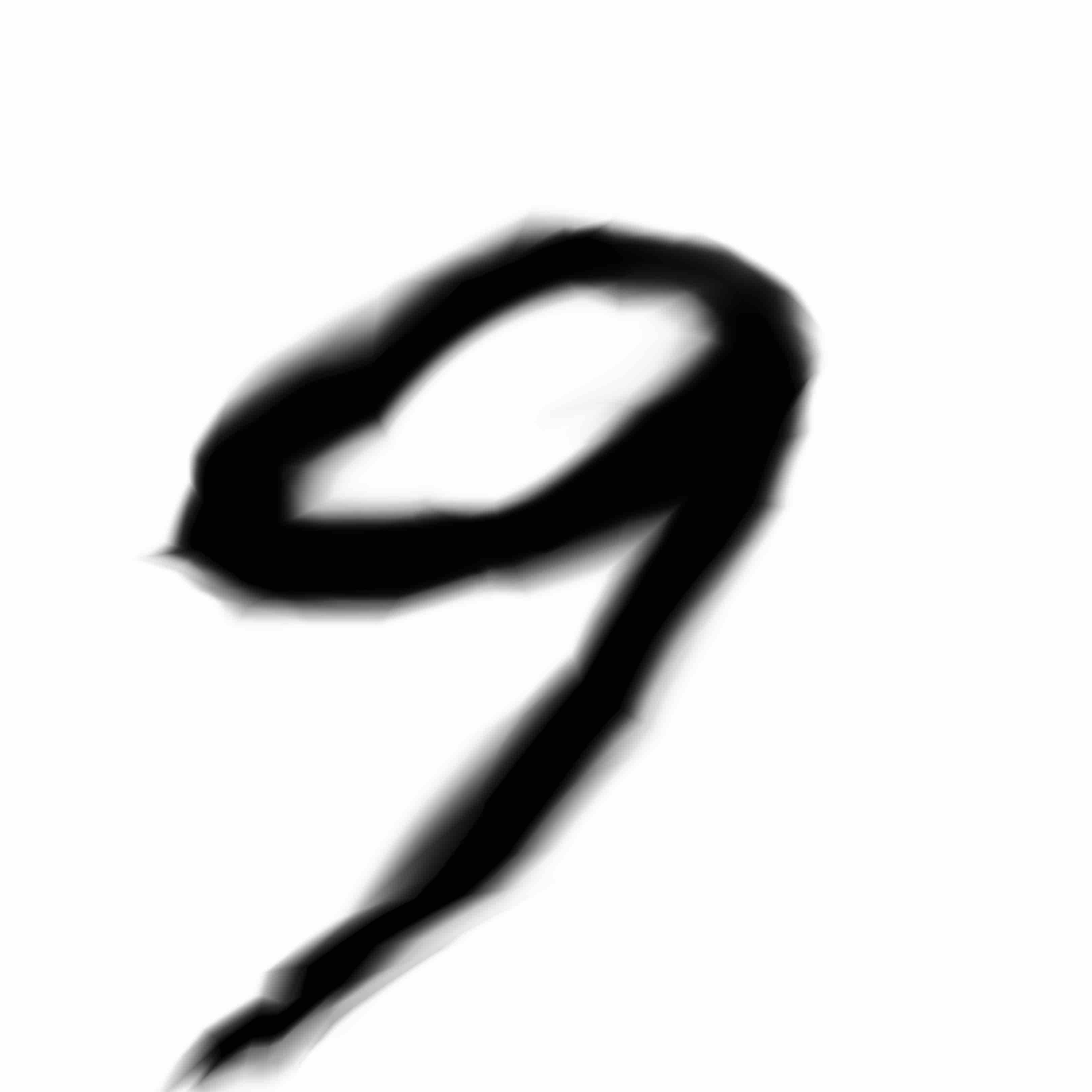
Below are the samples produced from the modifications from the model we will describe in this post:

I feel these newer samples are a lot more lively and express more character than the earlier ones produced from the previous model.

Model Description

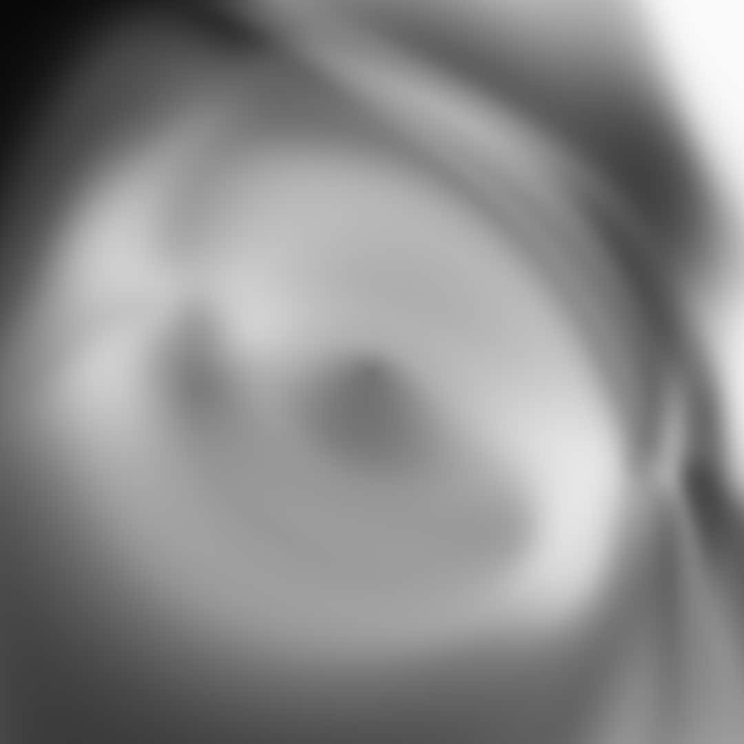
There are two goals that our generative model is to accomplish. The first goal is to train our generative network to produce images of MNIST digits that are indistinguishable from actual MNIST digits at 28x28 pixel resolution. The second goal is to use the same network to generate the images of the digits at a much higher resolution (ie, 1080x1080 or 3240x3240), and have the larger image actually look interesting to humans (well, to me at least).

We have seen a generative network create quite interesting images from purely random weights, so the thinking is training such a network to produce passable 28x28 MNIST images first, and then having the same network generate a much larger image might be able to satisfies our two goals.

Our generator can produce large random images of digits using random gaussian vectors as input.

The previous post describes how the entire model works. But unlike the previous model, this time we will make use of the classification labels for MNIST digits. At the beginning, a batch of training images will pass through a classifier network where this network will learn to recognise the actual digit label for each MNIST image (this is one of the first basic lessons of using neural nets for classification). Then, just like the previous model, the same batch of images goes into an encoder, to be converted into a bunch of gaussian random variables, called the latent vector Z, and that is fed into the generator network to produce another set of images.

Unlike the previous model though, the generated images do not necessarily have to look exactly like the set of training images. All the generator has to do is to create a set of new images that share the same classification labels of the set of training images. In other words, the generator network’s job is to will fool the classifier network to think that the generated images are of the same class as the original batch labels.

In addition to learning to classify digits, the classifier network also then learns to detect fraudulent images generated earlier and must learn to put those fake images in its own class (so there will be an 11th category in Softmax, after 0-9 labels).

Replacing Discriminator with Classifier Network

The classic GAN model used a binary discriminator to tell if a generated image came from the set of real training images or not. The discriminating function is a relatively easy machine learning task, and quite easy to train.

The problem we encountered is that the pure GAN model will tend to produce only a subset of MNIST digits really well to pass the discriminator test. No guarantee that all 10 digits will be generated. If the network is really good at generating the numbers 4 and 6, it won’t bother with producing 7’s. This is why I moved onto adding a VAE component in the previous model to force it to generate the entire set of numbers via the VAE training process. However, that is not the only method to force a diverse set of images the network can produce.

In this model, in order to get the network to generate all ten digits, the discriminator network is converted to a classifier network. Softmax is used to assign the classifier’s output probability that a given image belonging to a certain digit class. The generator’s job is to then try to generate an image given latent variables belonging to a certain class of digits, ie, maximise the probability of the classifier’s softmax output for that class. Not only does it have to generate an authentic MNIST digit, it must generate an image that looks like a certain class. The classifier will have to learn to detect fake images and put them in the 11th class, in addition to learning to classify the images from the training set into 0->9 labels. By adding this condition, our GAN model will have no choice but to be able to generate all ten digits, since that is what it is being tested on constantly. This is a similar concept as Style GANs incorporating extra information labels into the images the network is to produce.

The goal of the discriminator network is to maximise the below 2 conditions:

P(Classifier Output = Training Label | Training Image)
P(Classifier Output = Class 11 | Generated Image)

The goal of the generator network is to maximise:

P(Classifier Output = Training Label | Generated Image)

While at the same time minimising the latent error.

Variational Autoencoder Loss Function

Original, the VAE served two purposes: to encode a sample image from the MNIST dataset into a small vector of real numbers that look like unit gaussian variables (a latent vector 32 numbers in our model), and also produce images that look similar to the training images.

Difference in the Gaussian-ness of the latent vectors vs a real Gaussian is called the latent loss, or KL divergence error. This error can be easily calculated end-to-end via back propagation using black magic tricks taught to us mere mortals by the Bayesian Gods.

The similarity measure VAE calculates is based on pixel-by-pixel differences between generated vs original images. To calculate this pixel-by-pixel reconstruction loss, it can use either L2 loss, or logistic regression loss, and this error can also be minimised via end-to-end back propagation training. The total loss of the VAE is the sum of both both reconstruction loss and the latent loss.

I’m not a fan of pixel-by-pixel reconstruction error because that is not how humans look at the world. When we see a photo of a dog, we don’t compare pixel-by-pixel to some memory in our brain to determine whether the photo is indeed a picture of our pet dog, but rather compare abstract higher order features and concepts extracted from the photo.

If the convnet classifier used to classify an image into correct digits described earlier is also learning to extract higher order concept and features from images, it would be more interesting to use this convnet to tell us how good our image is, instead of pixel-by-pixel reconstruction loss. So in this model, we will replace the construction loss by the classifier’s loss function used in the earlier section to minimise the softmax error instead.

As a bonus, we can train generative model and VAE latent error together in one step! No need to do it in two steps like the previous model. I found that this process simplifies generative model training, and at the same time giving more work for the discriminiator-classifier to do. The discriminator has the extra task of learning to classify digits in addition to telling real from fake. It was a big problem in getting GANs to train well, as we always need to slow down the discriminator’s training to give the generator a chance. The gap in difficulty also narrowed a bit, making the GAN system easier to train.

Description of Generator Network

The generator used in the previous model uses 4 large layers of 128 nodes that are fully connected. This made it relatively easy for the network to fit a variety of training data, but I found that larger networks do not necessarily result in more interesting images.

Thinner but Deeper network

I found that smaller networks with deeper architectures, if the weights are set appropriately, look more interesting to look at compared to large shallow networks. Maybe this is related related to how deeper networks are exponentially more computationally capable compared to shallow ones. However deep networks are more difficult to train. Recently there are some discoveries such as residual networks that makes it easier to train very deep nets.

Residual Components

I chose to use a residual network architure to train a very deep but thin generative network. The residual nature of the network makes it easier for gradients to backpropate errors across many layers. The idea of using this architecture for the generative network was inspired by the DRAW model, which uses a same network block around a dozen times recurrently to additatively generate an image. I thought I might try using a residual network and having the flexibility for the weights for each block to be different.

Architecture of the Generator Network:

Architecture of Individual Residual Block:

In the end I used a stack of 24 residual network blocks, and each block contains 5 layers (4 relu and 1 tanh), displayed in the figures above. The heavier lines indicated that the initial weights will be large, while light lines indicate the opposite. The trick is to initialise these blocks so that they can generate interesting images.

Large Weight Initialisation

Typically in neural network training, the rule of thumb is to prefer a set of small weights, inversely proportionaly to the square root of the number of nodes, to avoid overfitting the data. At the beginning, weights are initialised to be close to zero, and the optimizer will penalise large weights from regularisation. I think this is a sensible way to train networks for classification or regression type problems.

Images generated 8 layers of 64 nodes. Weights randomly initialised as below:

stddev = 0.30	stddev = 0.45	stddev = 0.60

However, for image generation, smaller is not always better. We can see in the above figure that even at a standard deviation of 0.30, which is likely much larger than initial weights used for typical neural network training, the resulting image does not look too interesting. Images generated with a set of larger random weights look more interesting than smaller weights, and if the weight start out closer to zero, I found that they will only get large enough to solve to task at hand, but get no larger than that. I decided to initialise the weights of the relu layers inside each subblock to be much larger than usual (ie, with a standard deviation of 1.0), so that those blocks will generate more interesting subimages individually. The final tanh layer for each block, however, will be initialised to weights very close to zero. Since tanh(0) is 0, initially, each block of the resnet will just flow through like an identity function. The optimiser will increase the size of the weights of the final tanh gates for each subblock gradually letting it have access to interesting random properties of each of the 24 randomly initialised blocks.

This turned out to be important if I want to generate images that are not boring. I got the idea from reading about neural network research of the distant past, such as echo state networks, reservoir computing, and evolino LSTM training methods. The theory was that since back in those days large neural nets were difficult to train, what we can do is to define a very large neural net (can be feed forward, or even rnn/lstm) with totally random weights (or weights produced from neuroevolution). It turns out that neural nets with totally random weights can still have interesting and powerful computing capabilities. One thin final network layer is attached to a small subset of activations of the neural network to accomplish some task (such as predicting a complicated signal), and only this final thin layer is trained by back propagation. This hybrid random+trained layer turned out to be quite powerful for many tasks.

With our image generation, each tanh layer (with initially very small weights) can be trained to allow information from the heavy-weighted relu layers to pass through, thus allowing some of this randomness in the initial weight settings to appear in the final image.

Results

Below is a grid of digits generated from the previous model, which uses the reconstruction loss component in VAE:

Here is a grid of digits after 6 epochs of training in the new GAN model with the residual generating network. If you click on an individual image, there are visible differences in the finer details compared to the previous model.

I also experimented with using a generative network with only 4 nodes per layer. We can see some constraints and struggles when it tries to generate all 10 digits:

I also trained the model much longer than 6 epochs, and I found that after 24 epochs of training, the network does a much better job at producing better MNIST digits, but however this comes at the expense of how interesting the images look after they get blown up to high resolution. Perhaps some of the large initial weights were pushed lower over time to satisfy the first goal of the model, while sacrificing second goal of producing something that looks more interesting to me - I guess that is something that cannot be easily quantified yet.

Previous Model:

Current Model - 6 Epochs:

Current Model - 24 Epochs:

Which one do you like the most?

Citation

If you find this work useful, please cite it as:

@article{ha2016cppngan,
  title   = "Generating Large Images from Latent Vectors - Part Two",
  author  = "Ha, David",
  journal = "blog.otoro.net",
  year    = "2016",
  url     = "https://blog.otoro.net/2016/06/02/generating-large-images-from-latent-vectors-part-two/"
}