For the Javascript demo of Mixture Density Networks, here is the link.

Update: A more comprehensive write-up about MDNs implemented with TensorFlow here

While I was going through Grave’s paper on artificial handwriting generation, I noticed that his model is not setup to predict the next location of the pen, but trained to generate a probability distribution of what happens next to the pen, including whether then pen gets lifted up.  It eventually made sense to me, since if we train the model to predict the next location based on some mean squared error minimisation function the model would not get anywhere as the average of the next step may not contain much information.  The algorithm actually generated a gaussian mixture distribution used for predicting the next location of the pen, and also a simple bernoulli distribution for whether the pen stays on the writing pad or not.  It was a bit over my head as this concept is then combined with Long Short Term Memory neural nets and conditional gates for handwriting synthesis.

After a few discussions with Quantix who advised me to go through some useful literature, I became interested with an old paper about Mixture Density Networks approach developed by Bishops way back in the mid 1990’s, who now works for Microsoft Research.  I thought that the paper was very well written and the author’s style was more about teaching the reader how something works rather than promoting their research.  I wish more papers nowadays were written in the same style.

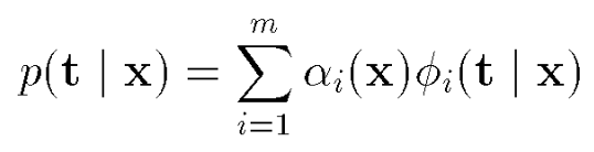
Mixture density models are nothing new and they are used everywhere to estimate the real distribution of some data, typically by assuming that each datapoint has some probability to be associated to a certain gaussian distribution, as in the equations below:

The mean square minimisation approach can be regarded as similar to the special case of the mixture gaussian model when m=1 (but not exactly the same).

This sort of model can be useful if combined with neural networks, where the outputs of the neural network are the parameters of the mixture model, rather than direct prediction of the data label.  So for each input, you would have a set of mean parameters, a set of standard deviation parameters, and a set of probabilities that the output point would fall into those gaussian distributions.

Bishop’s paper mentioned that often in machine learning problems, we have to solve inverse problems, and we are interested in learning about some state that get us the correct answer.  For example, given some medical symptoms, estimate a list of likely diseases that the patient may have.  Or, given a desired location of a robotic arm, figure out which angles should all the robotic joints rotate towards, so that the robotic arm can get to the desired location.  For those problems, the average of the possible answers is unlikely to be the correct answer, so training the algorithm using a mean square error method will not work.

The Mixture Density Networks paper outlines the method to estimate the conditional mixture density parameters given some input, by minimising the cross entropy of the distribution mentioned above.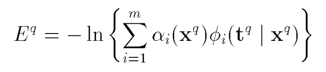

His paper included derivations on closed form gradient formulas making it possible to train the network efficiently using back propagation.  I attempted to implement his algorithm to tackle some toy problems.  As I wanted to make the algorithm work on a web browser, I used the graph objects from karpathy’s recurrent.js library for the implementation.  Note: there is actually no recurrent networks here, but I just liked how things are done in recurrent.js compared to the older convnet.js library, and features such as auto differentiation is possible, and in the future I can extend this code to do much cooler stuff.  You can click on the graphs below to see the training of the network done interactively in your web browser.

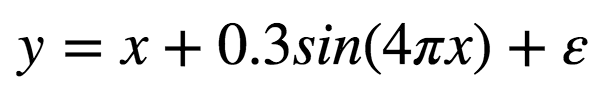
As a toy problem, we generate some random data, say based off this formula, a sinusoid with a linear bias and some gaussian noise, and try to get our model to fit the output.

The data can be easily fitted with a 2-layer network and 5 hidden tanh units (see demo here):

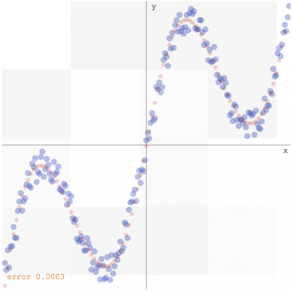
data fitting by minimising the square error

However, if we use the inverse of the data above, ie, the y’s become the inputs, and the x’s then become the desired outputs, we would have problems using the minimum square error approach, since for each input, there are multiple outputs that would work, and the network would likely predict some sort of average of the correct values.  If we run the same algorithm on the inverse data, this is what we get (see demo here):

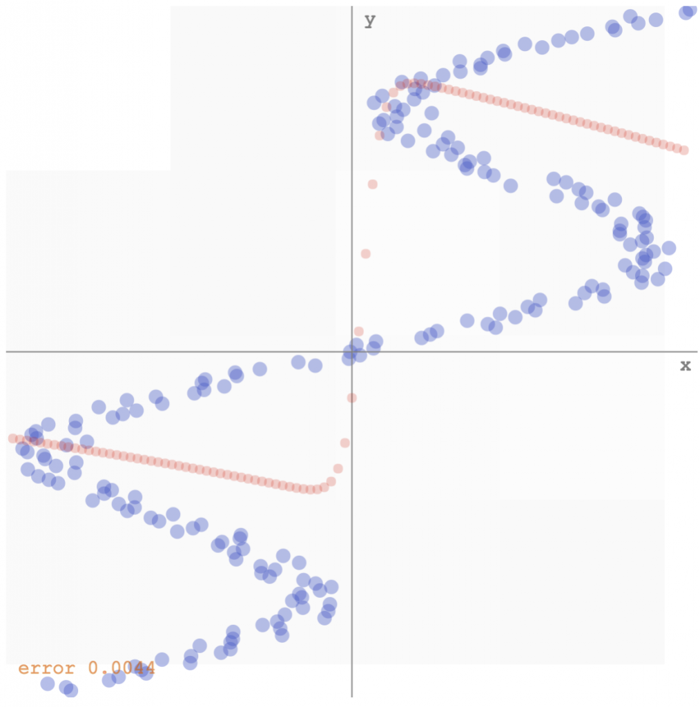
minimum square error data fitting of inverse data

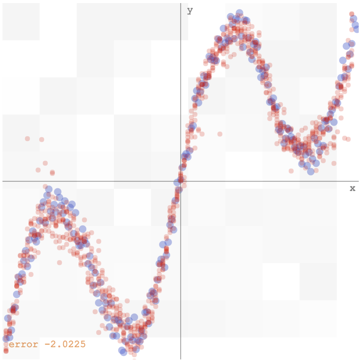
Bishop’s algorithm would have the network output a set of parameters for the gaussian mixture model, given each x value.  My implementation would sample ten values from that distribution, and plot those samples on the y-axis, to get a feel of the multi-modal distribution.  I have also played around with the number of mixtures needed to get it to work, and it seems that any value greater than 5 would do okay for this simple set of data.  Below is how the mixture density network model fits the inverse data (see demo here):

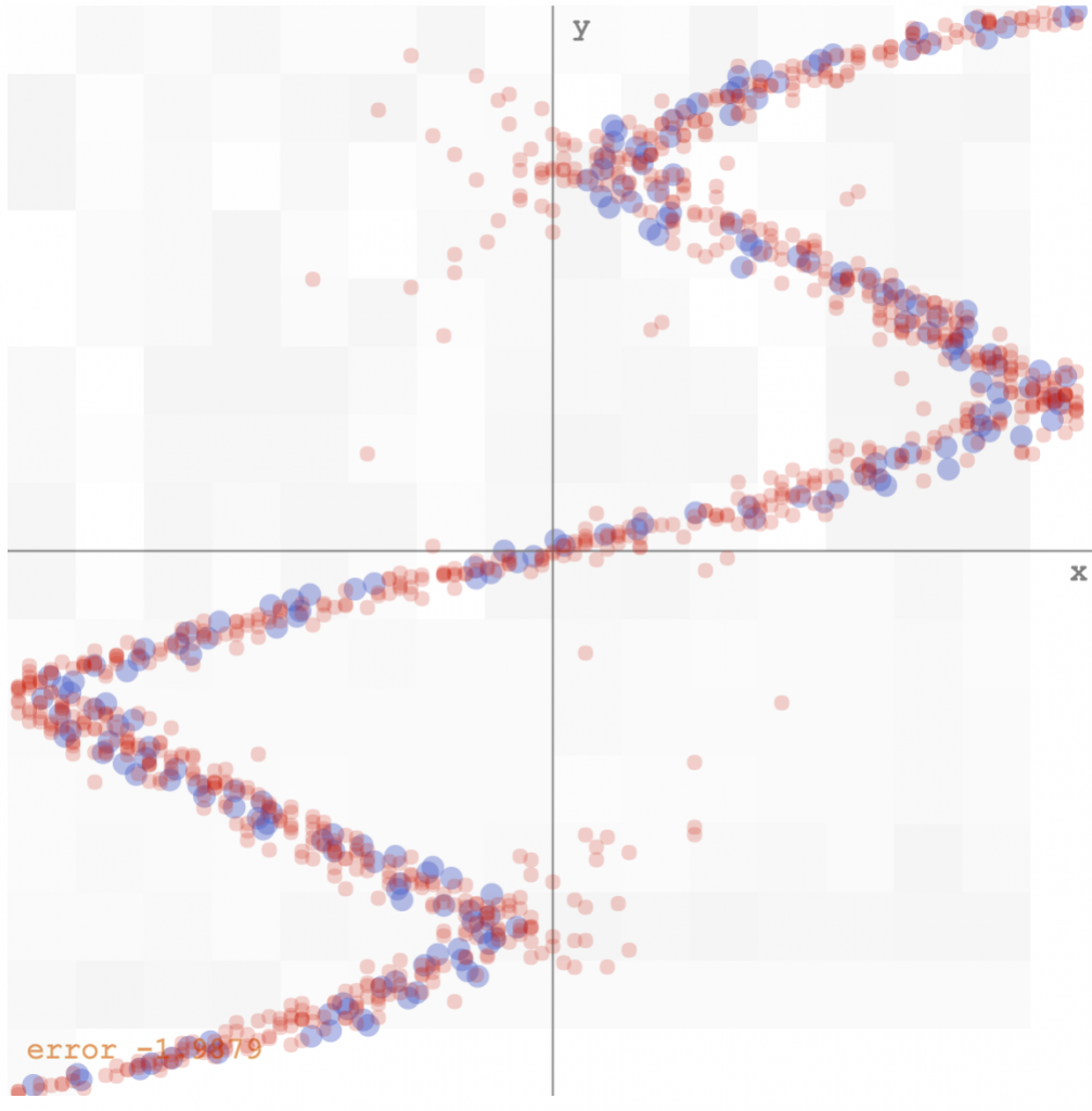
mixture density network predicting a distribution for the output, rather than a single value, for each input

We see that there are still some noise around the edges, and the convergence time is slower than the simple minimum square error approach, but I’m satisfied that it all actually works!

Just as a check, the mixture model would also get the original data set correct, although it is a bit slower, and would obviously be overkill.