Generative Model Combining CPPN w/ GAN+VAE.
GitHub
Introduction
In some domains of digital generative art, an artist would typically not work with an image editor directly to create an artwork. Typically, the artist would program a set of routines that would generate the actual images. These routines compose of instructions to tell the machine to draw lines and shapes at certain coordinates, and manipulate colours in some mathematically defined way. The final artwork, which may be presented as a pixellated image, or printed out on physical medium, can be entirely captured and defined by a set of mathematical routines.
Many natural images have interesting mathematical properties. Simple math functions have been written to generate natural fractal-like patterns such as tree branches and snowflakes. Like fractals, a simple set of mathematical rules can sometimes generate a highly complicated image that can be zoomed-in or zoomed-out indefinitely.
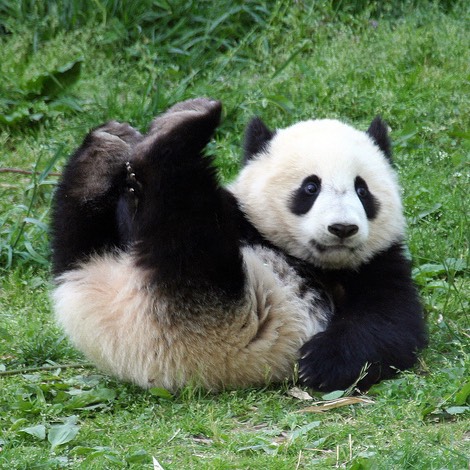
Imagine if you can take any image, and rather than storing that image as a set of pixels, you try to figure out a math function to approximate that picture, ie:
Once such a function is found, then the image can be automatically scaled up and down, or stretched around, by just scaling the inputs. If this function has some fun properties or exhibit some internal structure, it will be interesting to see what the image looks like if we blow up the image to a very high resolution much bigger than the original image.
This function can also be defined as a neural network, with arbitrary architectures. These networks, which some call Compositional Pattern Producing Networks are a way to represent an entire image as a function. Since neural networks are universal function approximators, given a large enough network, any image of finite resolution can be represented using this method.
|
|
Train a neural net to draw an image with karpathy’s convnet.js demo.
I think the style generated by neural nets of various architectures look really nice, so I wanted to explore whether this type of generative network can be used to generate an entire class of images, not just a single image, and see if I can use this method like the way recent research work used neural nets to generate pixellated images of a certain class.
In this post I will describe my experience of using CPPNs to generate high resolution images of handwritten digits, by training it on MNIST (28x28px), as a starting point. In the future I may try to use this method on more complicated image sets.

|
Background
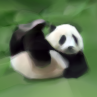
In the previous post, we have explored the use of CPPNs to produce high resolution images containing some interesting random patterns. Since the input to the CPPN consist of the coordinates of a certain pixel, and the output is the colour for that coordinate, CPPNs can generate images of arbitrary resolution, limited by the machine’s memory. This feature gives CPPNs some fractal-like characteristics, because you can just zoom-in, or zoom-out of an image as much as you want, by just adjusting a set of scaled input coordinates of the desired view of the image. We also find that by randomising the weights of the CPPN, we see that we can generate many abstract patterns that may look aesthetically pleasing to some people. Also, if we fix the neural network architecture, and fix set of random weights, we can explore the space of images that the CPPN can produce by varying around the addition latent vector input into the network.
Imaged generated with an untrained network initialised with random weights.
This same network will train on MNIST dataset.
I have used CPPN implementations before to generate many weird images, and I am constantly surprised at the wide range of pictures this method can produce. In addition to randomly generating abstract art patterns, this approach has also been used for genetic art production. In previous projects, where the art is slowly genetically evolved, it has been observed that to produce the ‘best’ art is to abandon the objective of actually creating a particular thing. For example, if an artist wants to use CPPN-NEAT to generate a picture of a cat, she would most likely not end up with anything that resembles a cat. But if the artist goes about choosing patterns that she thinks look interesting, and mix them up to produce the next generation of images, she might end up with something that looks even more interesting. Ken Stanley has highlighted this phenomenon in his work on Novelty Search, which I found to be a very fascinating approach to look at the AI research field, and also how to approach life in general.
However, I do think it is possible to get CPPNs to generate specific desired images. Given a large enough network, rather than a dinky little NEAT network, we can approximate anything, and even karpathy’s simple JS drawing demo proves that this approach can draw any image given a large enough network and enough training time.
The more interesting task though, is rather than to generate a specific image by overfitting the network’s weights to match some target image, is whether this sort of network can generate new images of concepts. For example, we want to be able to have the network generate a random picture of a cat, and be able to slowly morph that cat into a dog. That way, the network is not really overfitting to some particular training picture, but understands internally the concept of a cat and a dog, to the point where it is able to imagine a new image that is between a cat and a dog. A few years ago I thought this would be considered science fiction, but we are actually getting there.
Recently, we have seen deep neural networks capable of generating images of humans, bathrooms, cat, and anime characters. These approaches model the pixels in the images as observable random variables, X. Unless the set of pictures is of something very trivial like a white wall, the joint probability distribution of all the pixels inside X is a very complicated one that is unlikely to be modelled with simpler distributions understandable by mere humans. However, it is possible for a neural network to do the hard task of learning how to map this complicated distribution into a simple one that humans can understand and work with, such as a gaussian distribution. So the trick is to then model such complex observable random variables (all the pixels in an image) as a dependent variable, who’s value depends on a much smaller set of variables with a simpler probability distribution, like a vector of a dozen unit normal gaussians. This vector is typically denoted as Z, the latent vector.
So the goal is to have a neural network learn figure out the conditional probability distribution P(X|Z) to be able to generate a very complicated image X, from a very simple latent vector of real numbers, Z. In addition, having a complimentary network to learning P(Z|X) will also be very useful, to encode a complicated image to a latent vector.
If you think back to your first course in statistics, this is related to Principal Component Analysis (PCA), where one can try to decompose a large set of observations into a small number of factors. And one can then vary those small set of factors to predict what will happen to the large set of observations. The only difference is while PCA is based on linear algebra and assumes the data can be explained as a linear combination of smaller factors, this approach of using neural networks will be able decompose the large set of observations in a highly non-linear way, making it a lot more powerful.
Current cutting edge techniques of image generation from latent vector are generally based on Generative Adversarial Networks (GAN) or Variational Autoencoders (VAE) or a combination of these approaches, and I will describe them later in this post. To get more information into these methodologies, please read about Deep Convolutional Generative Adversarial Networks (DCGAN), which is a is well known state of the art technique in this area, and the DRAW algorithm is a cutting edge extension of VAE. My study of this area is based off of carpedm20’s implementation of DCGAN, and also Jan Hendrik’s implementation of VAE, both using TensorFlow library. Their code and explanations contributed greatly to my understanding. I’ve also studied this work on combining both approaches, and used some tricks to stabilise the training of GANs.
In the current literature, the training dataset is typically composed of small images (such as 32x32px or 64x64, though I have seen 128x128 and 256x256 sets being used). To match with the training data, the generator network will have as many outputs as there are as many pixels from the training data. So typically, a network used to train on an image dataset with 64x64 pixels would output also 64x64 pixels directly. It is difficult for modern methods to generate images that have much higher resolution than 256x256, because the amount of memory required is likely to exceed the amount available on a modern GPU card.
In this post, we will use CPPN to generate large images from smaller images from the MNIST training set. Because CPPN’s can generate images of arbitrarily large resolution, I thought it would be neat to try to train a CPPN to generate images, in the same way that GAN and VAE approaches have been used, and just replace the generator network that generates all the output pixels directly, with an indirect way of generating the pixels via a CPPN generator. For training, we can just set the output resolution of the CPPN to be the same as the input. After the training, we can increase the resolution of the output image to see how the CPPN ‘fills in the gaps’ with it’s own internal style defined by the network. By setting the training resolution of the CPPN to be the same size of the training data, the entire training process can fit inside a modern GPU board.
Due to the indirect-coding nature of of the CPPN’s architecture, the space of possible images that can be generated will be quite limited, compared to a network that outputs all the pixels directly, so from that standpoint, training a CPPN proved more challenging, and took a lot more time than training a VAE or GAN model on the simple MNIST dataset. After we obtained some satisfactory results with the CPPN model combined with GAN and VAE on a simple dataset such as MNIST, we can think about testing this algorithm on more complicated image sets of real, coloured objects in the future.
Generative Adversarial Modelling
As discussed in the background, the challenge for image generation, is to be able to model the joint probability distribution of the pixels in the image. Once we have a realistic probability distribution of all the pixels, we can just sample from that probability distribution to generate a realistic image. However, because real images are very complicated and the probability distribution too nasty for humans to model, the trick is to use a neural network to transform a much simpler probability distribution that humans can understand (like unit gaussian random variables) into a distribution that resembles the true probability distribution for normal images in our training set. The complexity of the generated probability distribution will be limited by the complexity of the neural network’s architecture. In our case, the neural network that will generate an image will be a CPPN, like the one below:
Architecture of the Generator Network:

|
This is the same sort of network used in the previous post. The input vector Z is a vector of 32 real numbers that are drawn from unit gaussian random number generator, and all of them will be independent. The vectors x, y, and r are all the possible coordinates we want to compute the pixel intensity for in our image, so for an image size of (26x26), we will need to calculate a total of 676 pixel intensities, to form (32+676+676+676) inputs into the network. The important point to note is that each pixel intensity will be calculated from the exact same network with the same set of weights, so theoretically we can also feed into our network (32+1+1+1) inputs and get 1 pixel, and do this 676 times, without moving the weights, if we are constrained by memory.
As we have seen earlier, by keeping the weights of the network constant, and by controlling the input Z vector, we can get a rich set of output images using this method. The goal here is to train our network in a such a way that for any random Z vector we put in, the output would look like an image from our MNIST training set, and we would not really be able to tell them apart. If we are able to successfully do this, then we would have used the CPPN to model the probability distribution of MNIST images, and we can draw random images out the way we draw simple IID unit gaussian variables.
But how on earth can we train the weights of this network to convert a bunch of unit gaussian random numbers into a random MNIST image? Someone living in the year 2013 will think this is science fiction. But if you were not cutoff from the internet and stuck in a cave, you would have probably heard of the Generative Adversarial Network framework in the last few years. The concept behind GANs is introduce a Discriminator (D) network to compliment the Generator (G) network above.
Architecture of the Discriminator Network:

|
The job of the D network is to be able to tell whether or not an image belongs to the training set. So it will be used to detect fraudulent pictures of MNIST digits that are not legit and authentic MNIST digits. The job of the G network is to naturally attempt to generate an image of a random MNIST digit that can fool D to think that it is the real deal. If D is very good at its job, and can discriminate images at the level of human level performance, and if G is able to still fool D, then G would be able to generate a fake MNIST image that can fool humans, and our job is done.
I followed a similar approach used in DCGAN, and used three simple convolutional network layers. Convnets have proven to be great at image classification, and since the output of D is binary in this case (real/fake), this is an even simpler classification problem than digit classification.
The input to the D network is an image. The output of the D network, y, is a real number between zero and one. If y is close to one, then the D network strongly believes that the input image must be a legitimate MNIST digit, and if y is close to zero, then the D network strongly believes the image is not an MNIST digit, but rather a fraudulent attempt to fool and undermine its intelligence. If the output of D is close to 0.5, then the network is confused and sad, having loss its confidence in its ability to function as a normal neural network.
We can define these performance measures, or cost functions, to evaluate the performance of the generator network:
You can see that if the generator network is doing a really bad job, then the output value y from the discriminator will be a very small number close to zero, and the negative of the log of a very small number will be a very large positive number.
If the generator is doing a fantastic job, and kicking D’s ass, then the output value y will be a number close to one, and the negative of the log of a number approaching 1 (like 0.999) will be a number close to zero.
If the generator creates an image that causes D to be confused and can’t tell the difference, the output y will be a number close to 0.5, then will be a value close to -log 0.5 or around 0.69
Likewise, we can evaluate the performance of the discriminator in a similar way:
If the discriminator is doing a great job, both and will be a number close to zero. Conversely, if the discriminator is doing a poor job, both and will be a very large number. If the discriminator is confused, both and will be a number close to , so the D network will have trouble identifying both real and fraudulent examples. We define the loss function to be the average of both losses.
Given the loss functions above, it is then fairly straight forward to train the D network using backprop to learn to distinguish a real MNIST digit from a fake one, by adjusting the weights in the direction of the gradient that will make smaller after a batch of real examples, and fake examples freshly generated by G.
The generator network can also be trained via backprop as well by adjusting the weights in the direction of the gradient that will make smaller (thereby also making larger).
Note that training G is much more involved, because during back propagation, the gradients has to flow through the layers of the D network first, into each pixel that G has generated (so will be first calculated). Afterwards, the gradient of each loss derivative with respect to each pixel will then flow backwards into each weight inside the G network (). And because we are using a CPPN algorithm to generate the image, every pixel is generated by the exact same network with identical weights, just with different coordinates as the inputs. Since the weights are shared, the gradients flowing back from the pixel level to the weights will be accumulated to compute . This means if we are doing minibatch training for a set of images, training CPPNs means we will involve working with a batch within a batch, and it took a while for me to figure out how to implement this correctly in TensorFlow, as many default shorthands to ignore batch processing wouldn’t work anymore.
Training Both Discriminator and Generator Networks
At the beginning, both networks’s initial weights are randomised, so both are totally stupid and don’t know what they are supposed to do. The key is to make them train together and get better gradually over time.
Architecture of the GAN Setup:
|
|
|
|
As outlined in the GAN paper, we would take turns training G and D for each minibatch, so over time, both would get incrementally better at beating each other, and through this competitive process, both networks would be better at what they are supposed to do as a standalone network. Ideally, we want both and to hover around (so that the output is ). If the D network is a lot stronger than the G network, we would find that would stay near zero, and would stay at a very high number during the training, since any incremental improvement in G would be quickly outpaced by any subsequent improvement in D.
In practice, this is what tends to happen. D is a simple classification network and it is generally very easy to train a good classifier, especially if we use a few layers of convnets. It is easier to tell that something is real or fake, than to actually create a fake thing that looks real.
In real life, anyone can tell apart a real masterpiece from a fake piece of art created by an amateur. It takes a professional art forger with years of experience to be able to create a fraudulent painting that looks like the real thing. Art Forgery can be an extremely lucrative profession partly because it is so difficult.
Like a real counterfeit painter, G has a much tougher job compared to D. Creating content is hard, and even with the error gradients advising G how to defeat D, there’s no real guarantee that G can do a much better job at fooling D. Sometimes the gradient can just be stuck at zero, when D has gotten good enough at winning that any small change in G’s strategy will not beat D.
One of the most important points of training a GAN network is to not let the discriminator network become that much better than the generator, so a lot of thought should be placed on structuring the architecture, and size of both networks so that they are fair. For example, the learning rate for G’s weights are larger than the learning rate for D’s weights.
In addition to the consideration for D’s network architecture, the number of activations for network D should be set to a low enough level so that it won’t improve to the point where G has absolutely no chance to trick D. At the same time though, D should have enough neurons so that its general performance should be comparable to a human doing the classification herself, otherwise even if G can outsmart D, the pictures it generate will not fool the human viewer. Therefore, at the end of the day, network G must have enough capacity to generate a large space of possible images. If G can only draw a simple circle, there’s no way it can fool any reasonable network with any amount of optimisation used to fine tune its weights. You can’t beat a dead horse.
There are some more tricks to slowdown D’s training so G can have a good chance to always catch up to D. This includes running gradient descent learning on G, N times for every time gradient descent learning is run on D, during every batch. We have experimented with setting N between 4 and 8 times.
Another trick is to calculate D’s loss function first, and only perform gradient descent on D if G’s loss function is less than some upper bound (so it is relatively not that weak against D in the first place), and also if D’s loss function is greater than some lower bound (so that it is not relatively that strong versus G). We have tried to use an upper bound of 0.80 and a lower bound of 0.45.
I have read about some of these tricks on this great post on training GANs, and also about how to combine GANs and VAEs that I will also discuss later. After these tricks are used, and fine tuning the architectures of both networks, we should see both loss functions of D and G hover around during batch training, so one network doesn’t become that much stronger than the other, while both incrementally getting better at their respective tasks.
GAN algorithm for 1 epoch of training:
1
2
3
4
5
6
7
8
9
10
11
12
13
14
15
16
17
18
19
20
Randomise Sample Images in Training Set
For each Sample Image in Training Set
y_real = Discriminator(Sample Image, w_d)
For i: 1 .. N_handicap
Z = Normal(mean = 0, stdev = 1, Size=(1, N_z))
Image = Generator(Z, w_g)
y_fake = Discriminator(Image, w_d)
Calculate G_loss
Calculate dG_loss/dW_g gradients via backprop
#i.e., the direction to make D crappier
Adjust W_g's using SGD-type optimising step
Calculate D_loss
if G_loss < th_high and D_loss > th_low
Calculate dD_loss/dW_d via backprop
#i.e., the direction that would make D better
Adjust W_d's using SGD-type optimising step
In our settings, N_handicap had been set to values between 4 and 8. th_high and th_low had been set to 0.80 and 0.45 respectively. The architecture and specification of the networks are similar to the setup in the reference github code.
The MNIST training data had resolutions of 28x28 pixels. We have cropped them to 26x26, and randomly sampled between coordinates (0, 0) -> (25, 25) to (2, 2) -> (27, 27) so we have four times more variety in our training samples. This might not benefit the current version of the GAN algorithm, as the D network is a convnet, but in the next few sections, when we merge GAN and VAE, it will offer some benefits to the VAE side later on.
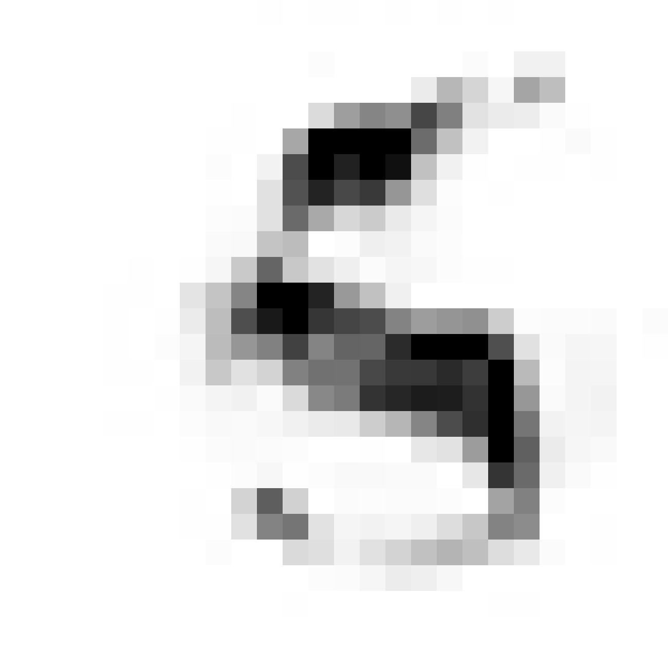
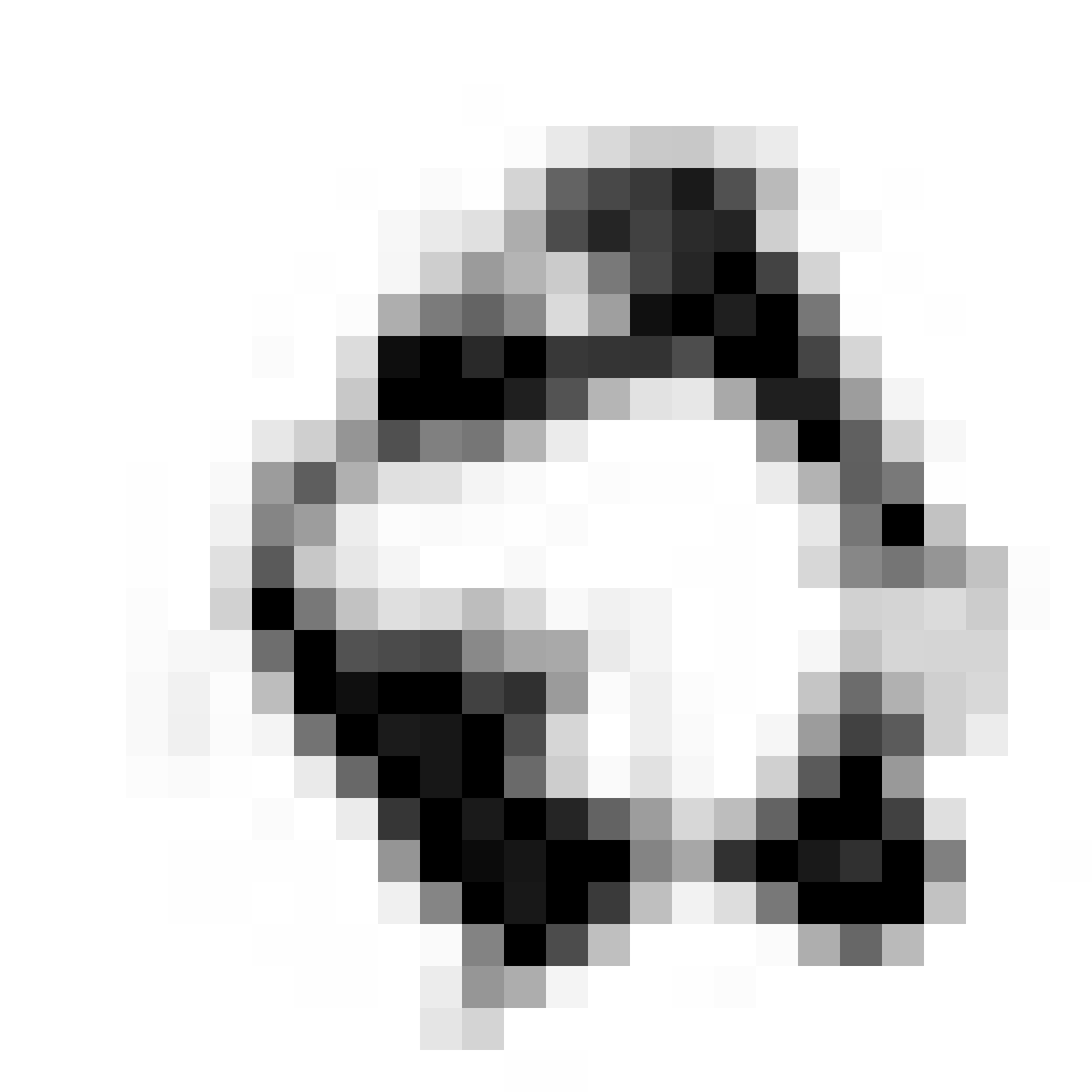
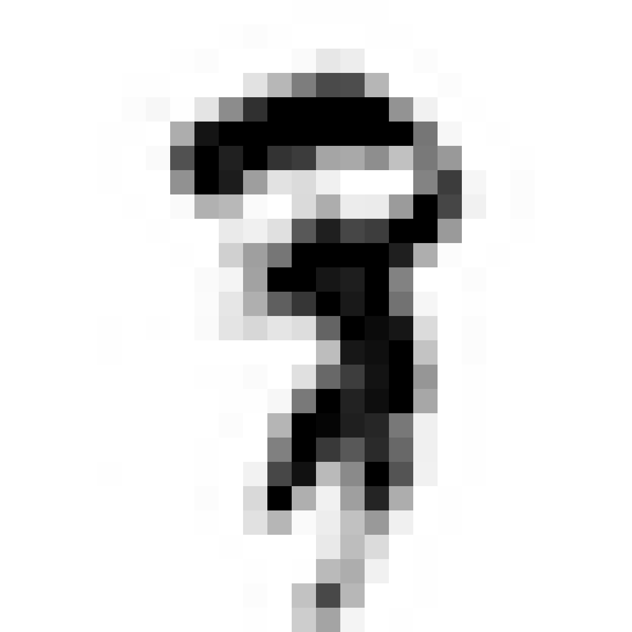
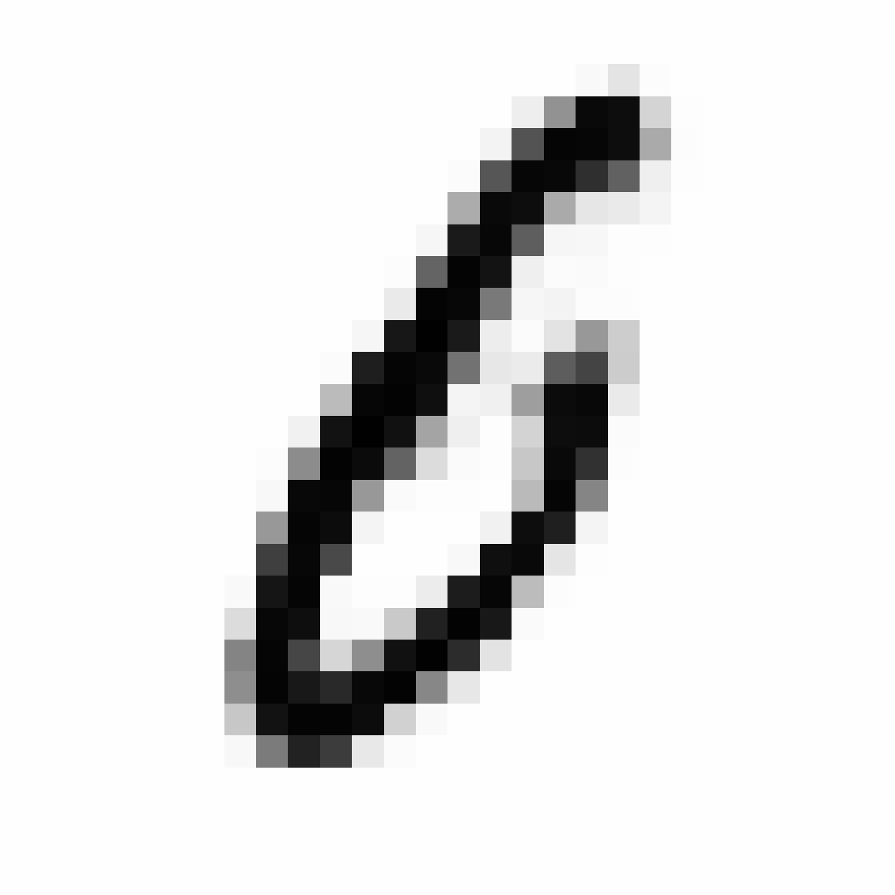
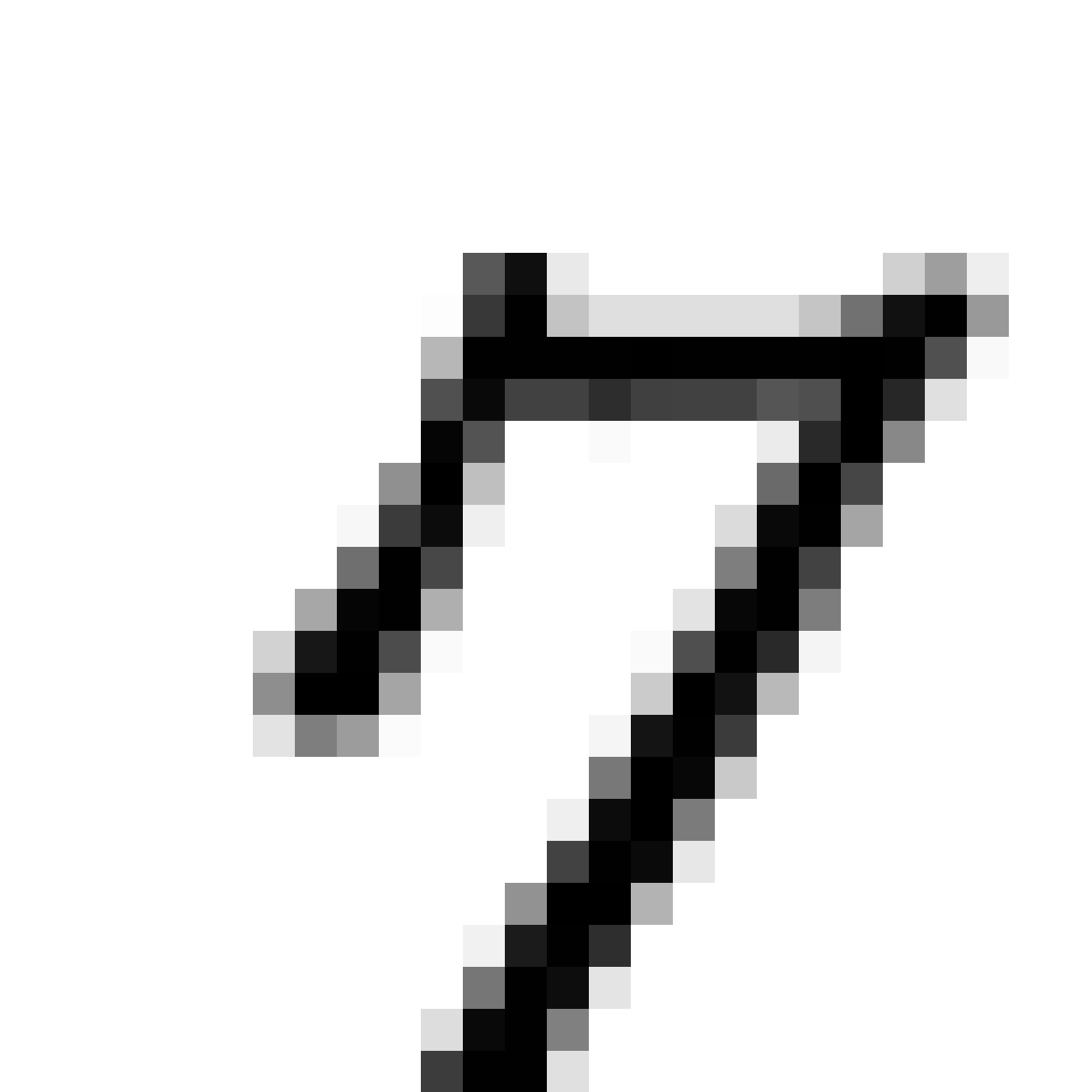
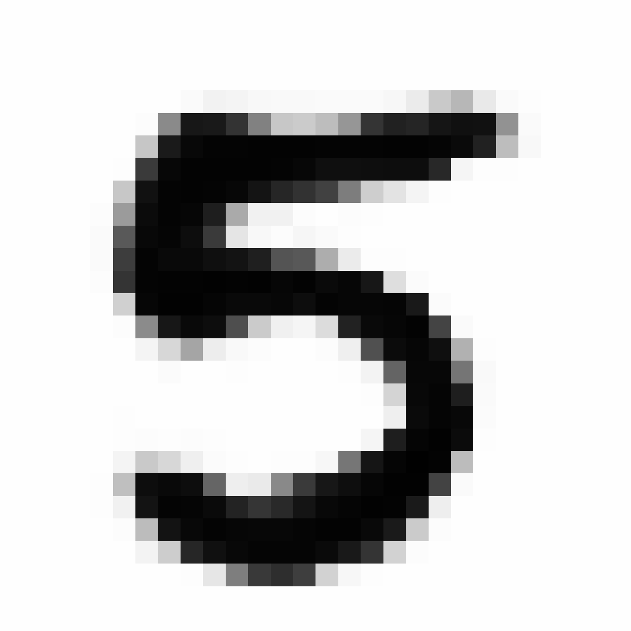
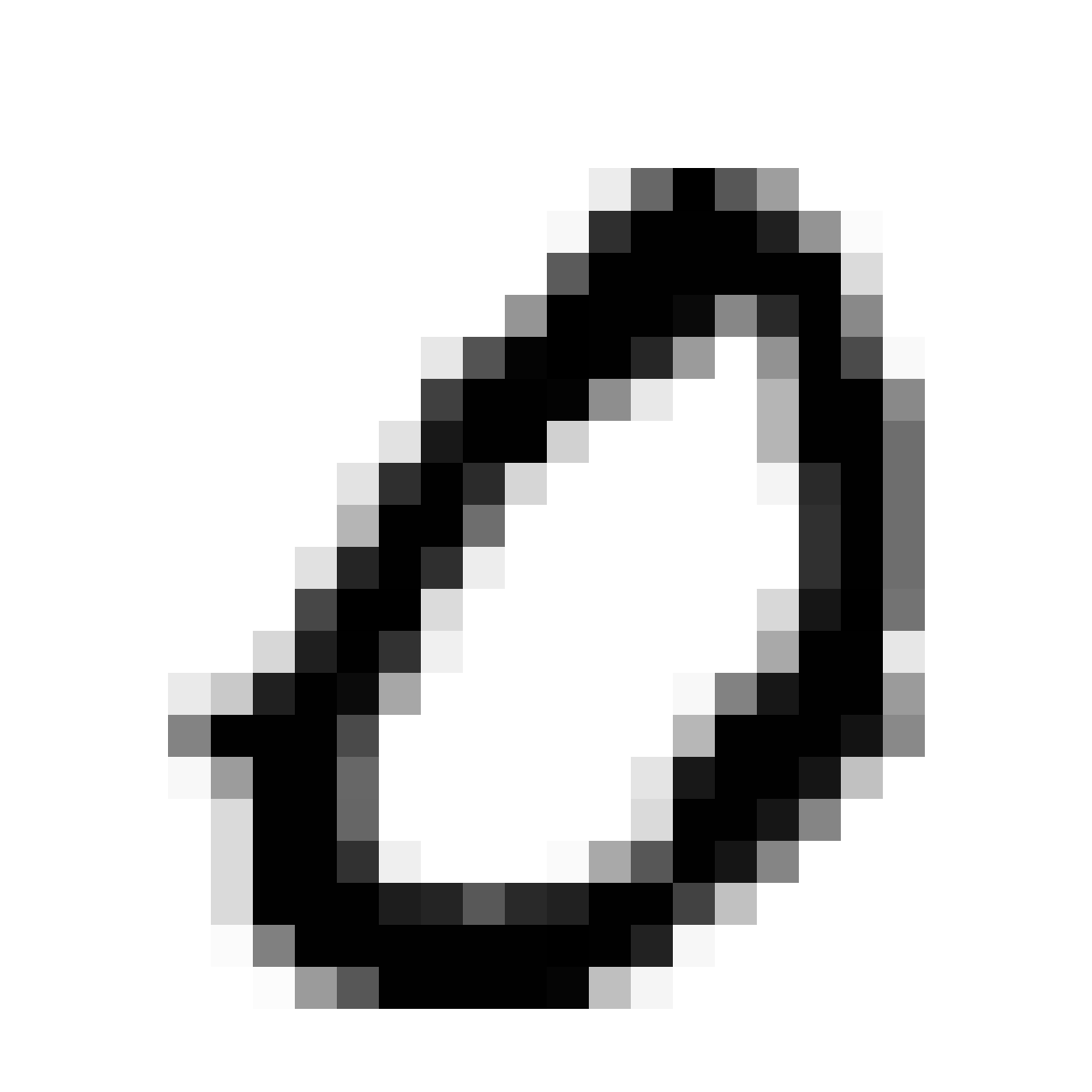
Samples of generative network at 26x26 output resolution:
|
|
|
In the figure above are are a few examples generated from the G network after a few epochs of training using this GAN method. The images resemble MNIST samples at 26x26 resolution. We get images that sort of resemble zero, five and nine digits.
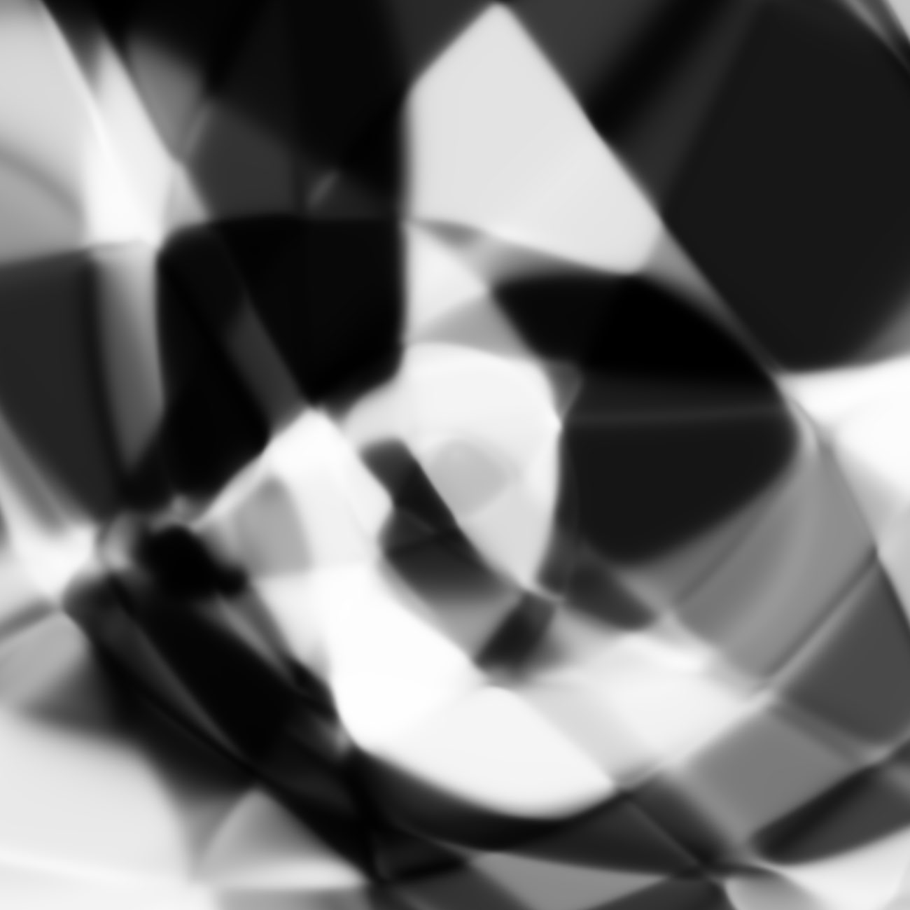
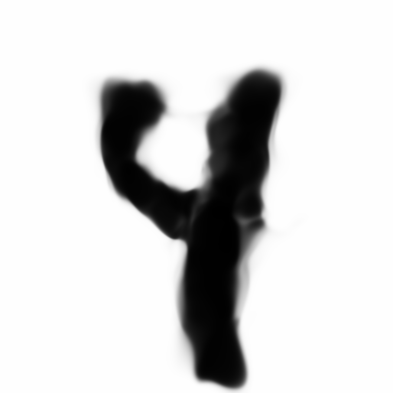
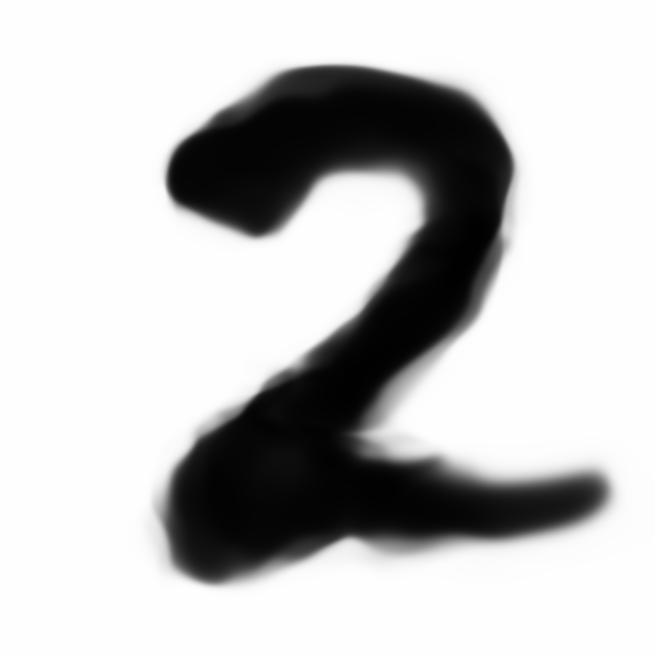
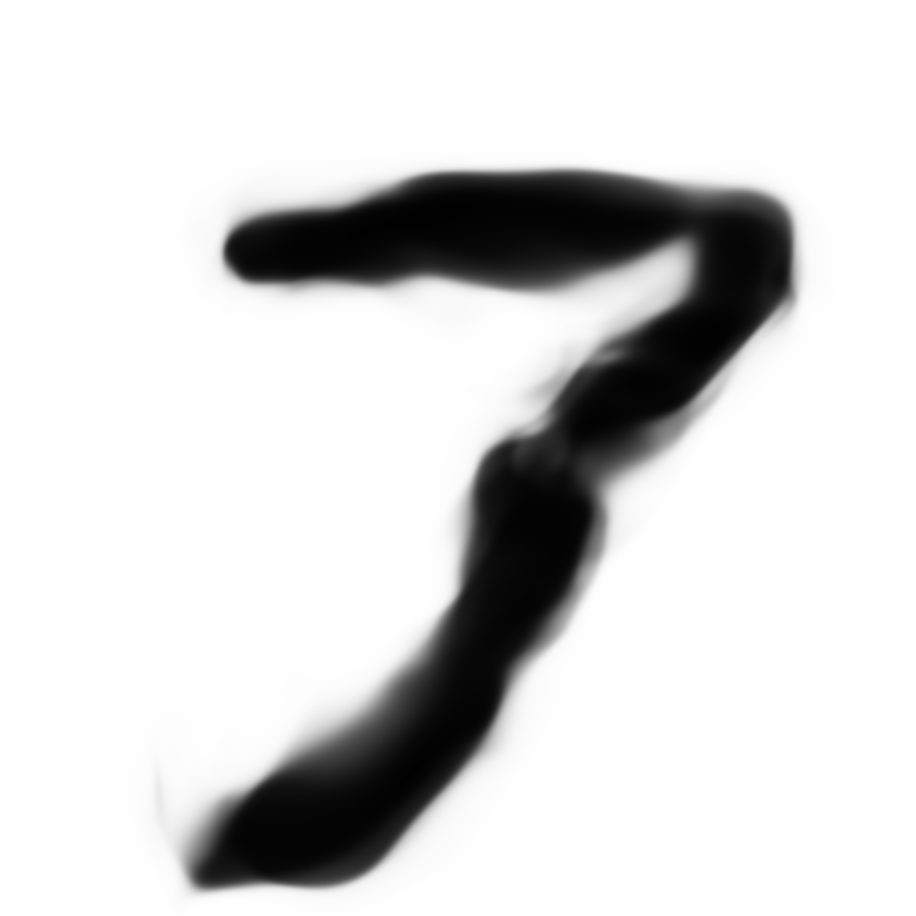
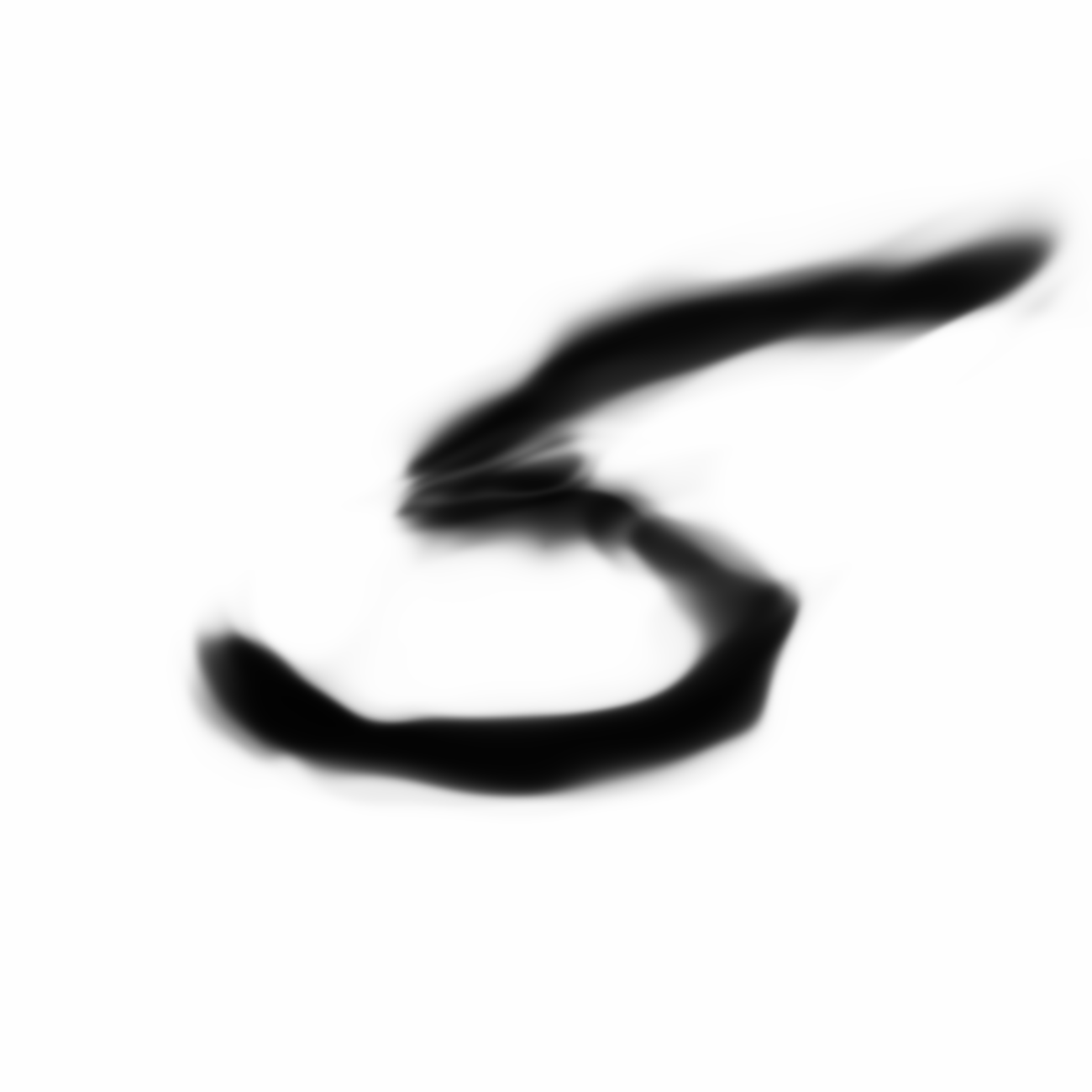
Now let’s see what happens when we use the CPPN network to blow up the images using the same latent vectors to generate a 1300x1300 resolution image.
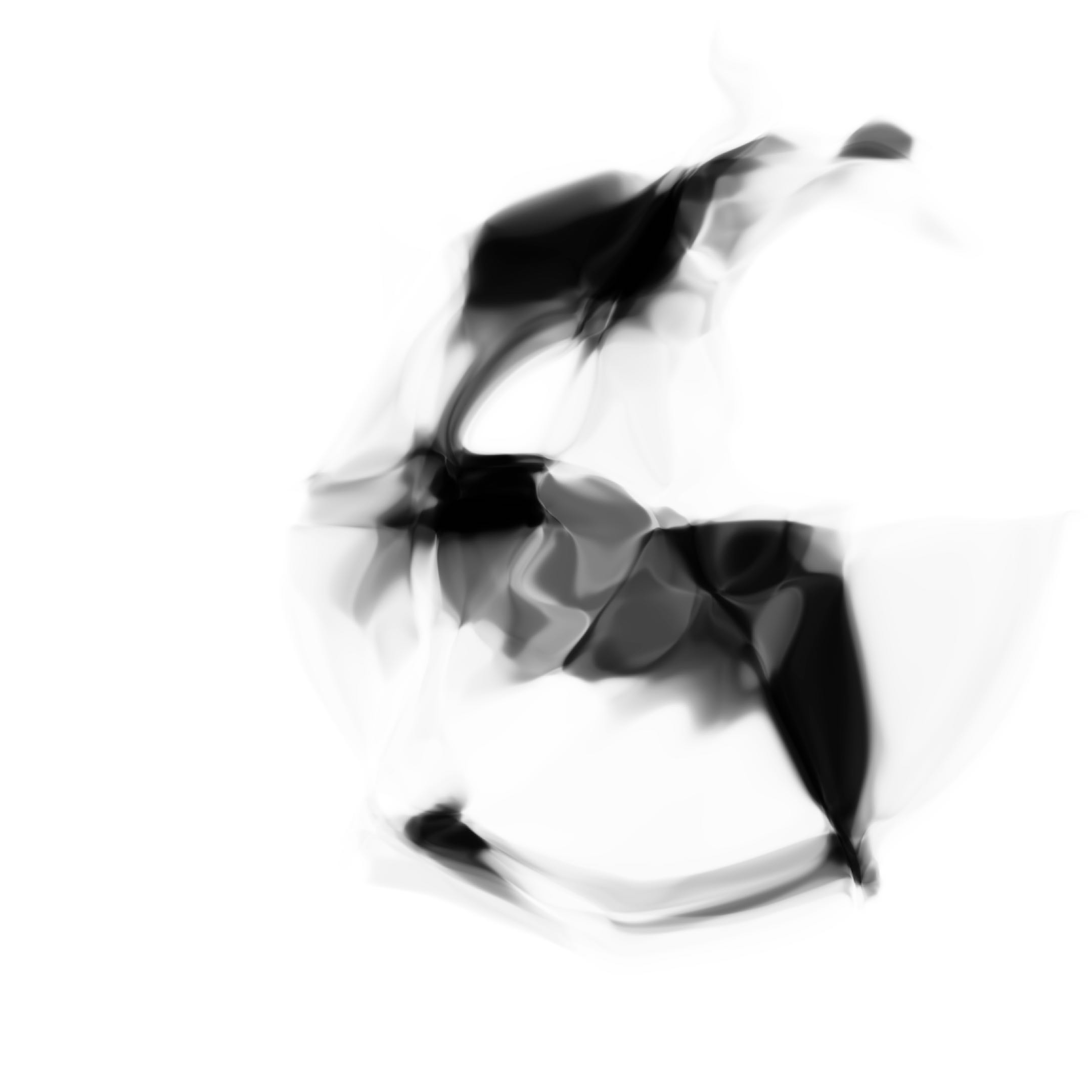
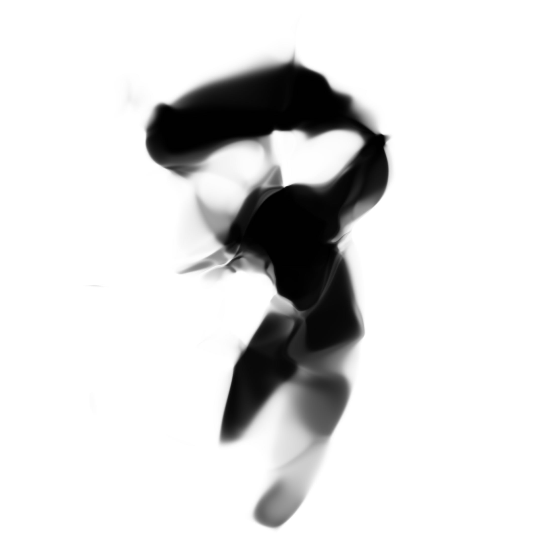
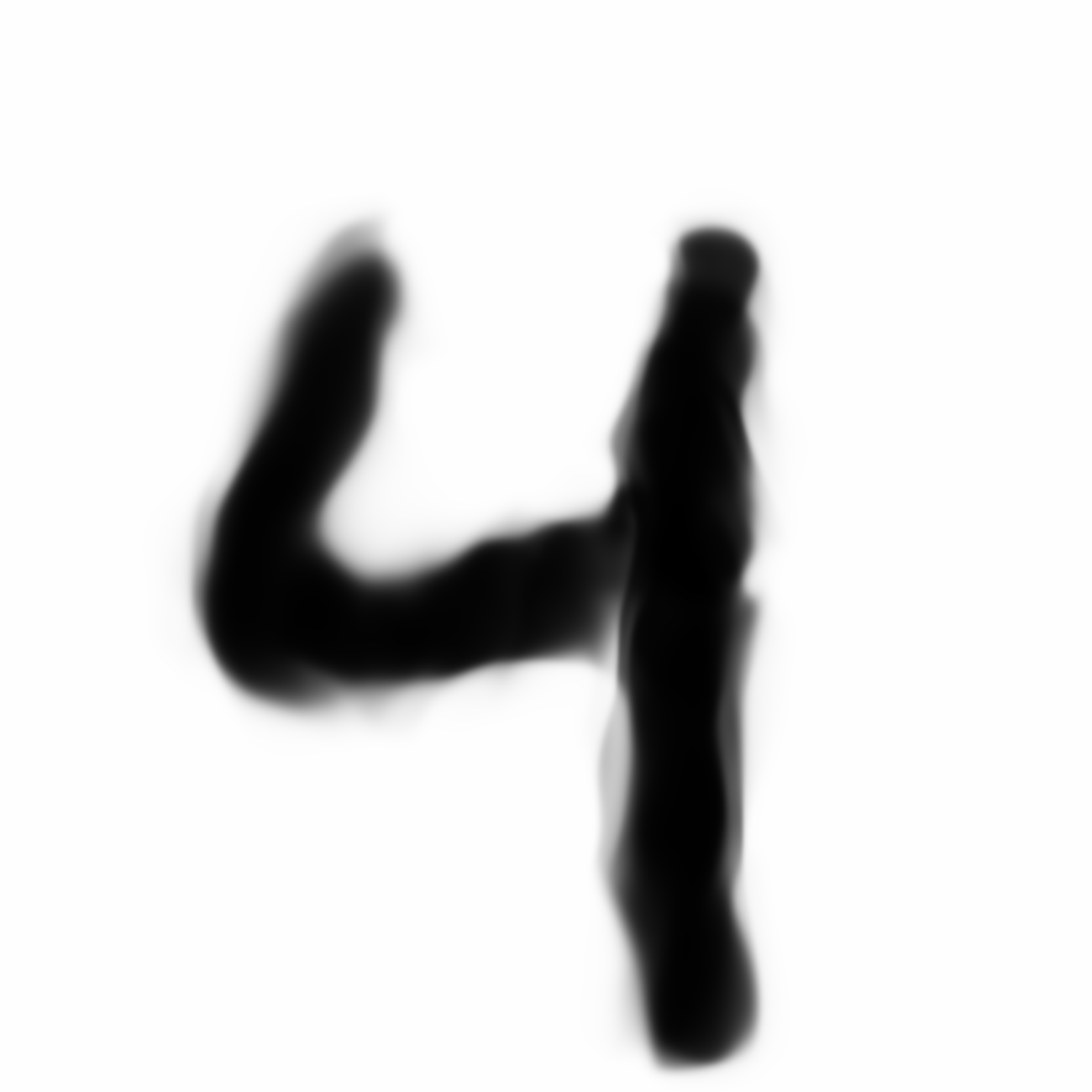
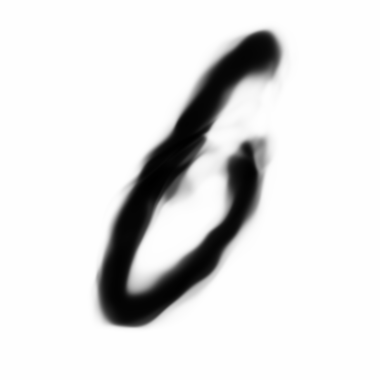
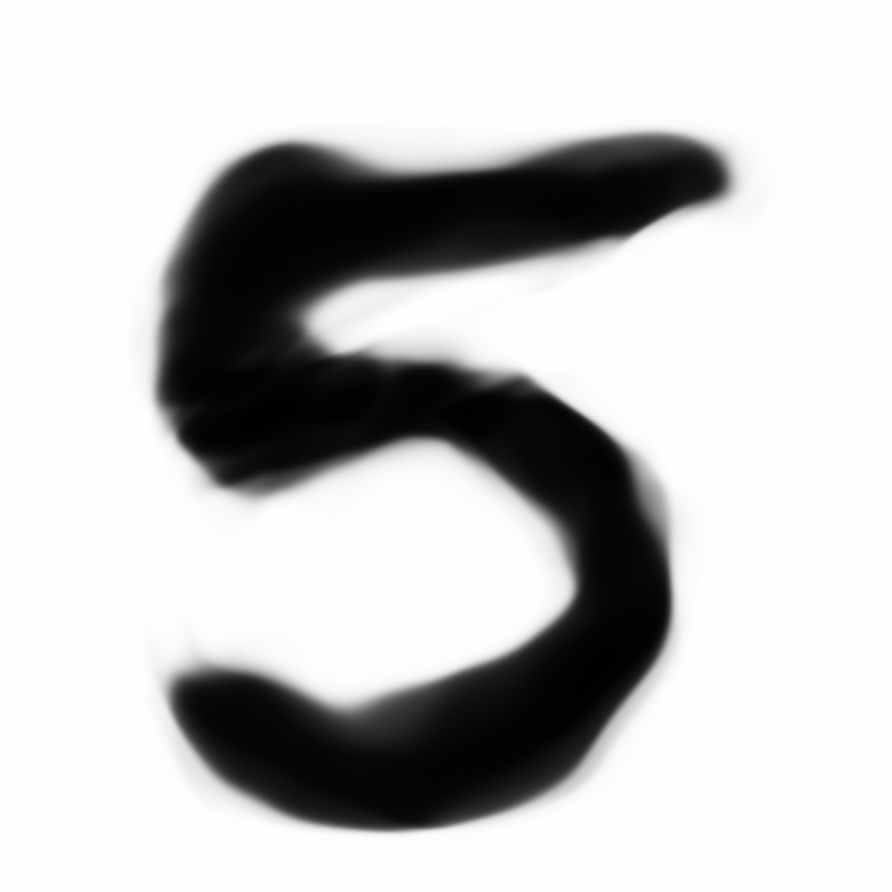
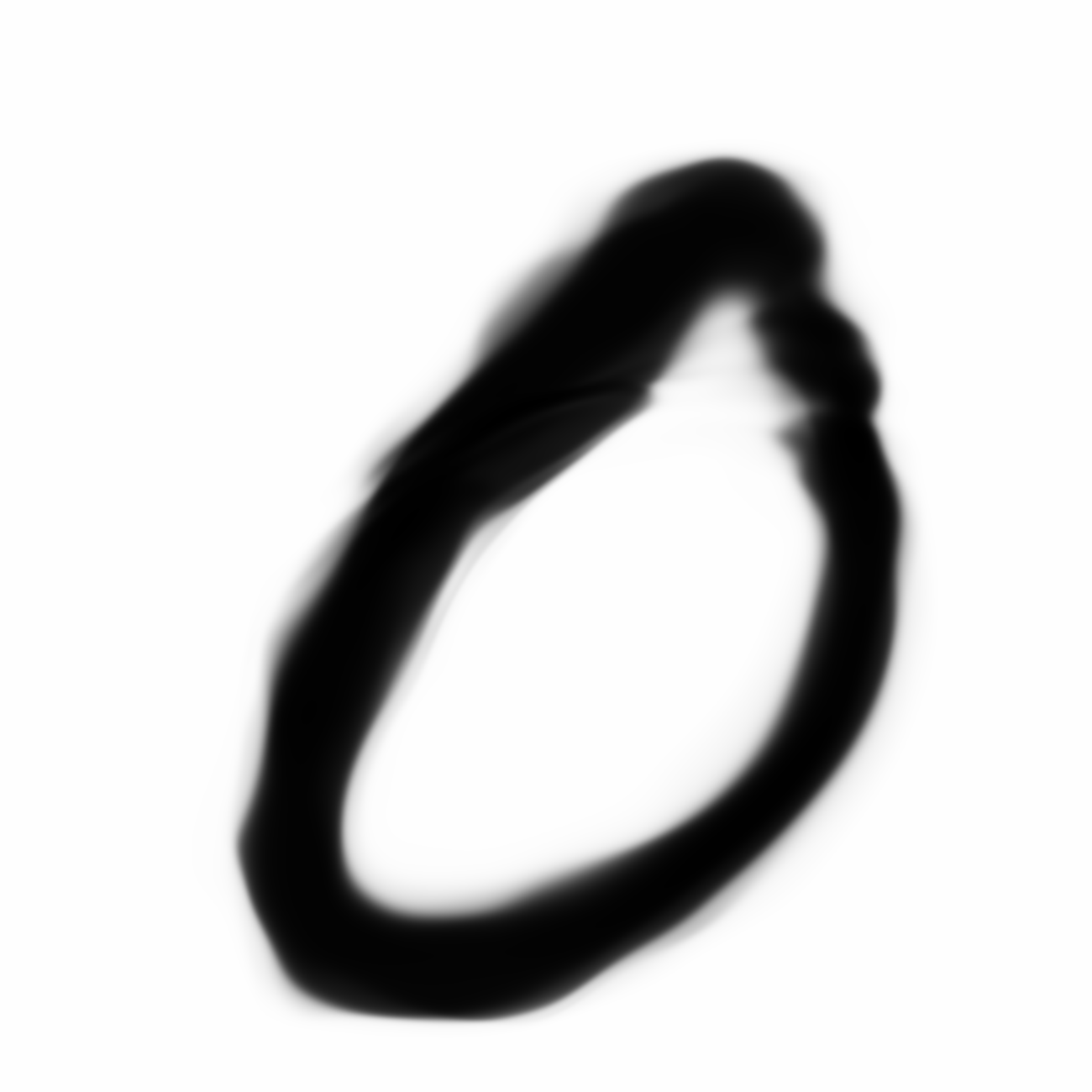
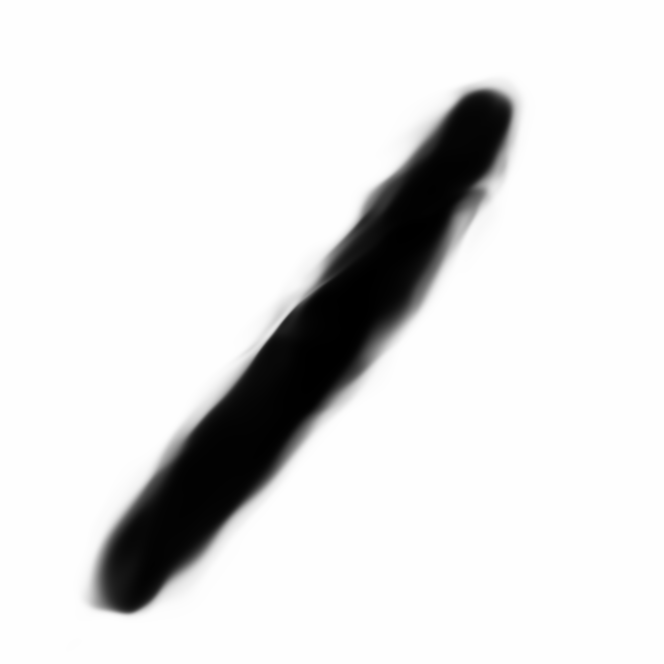
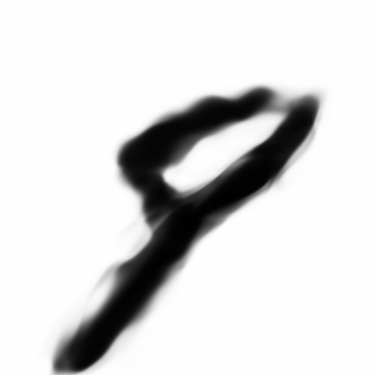
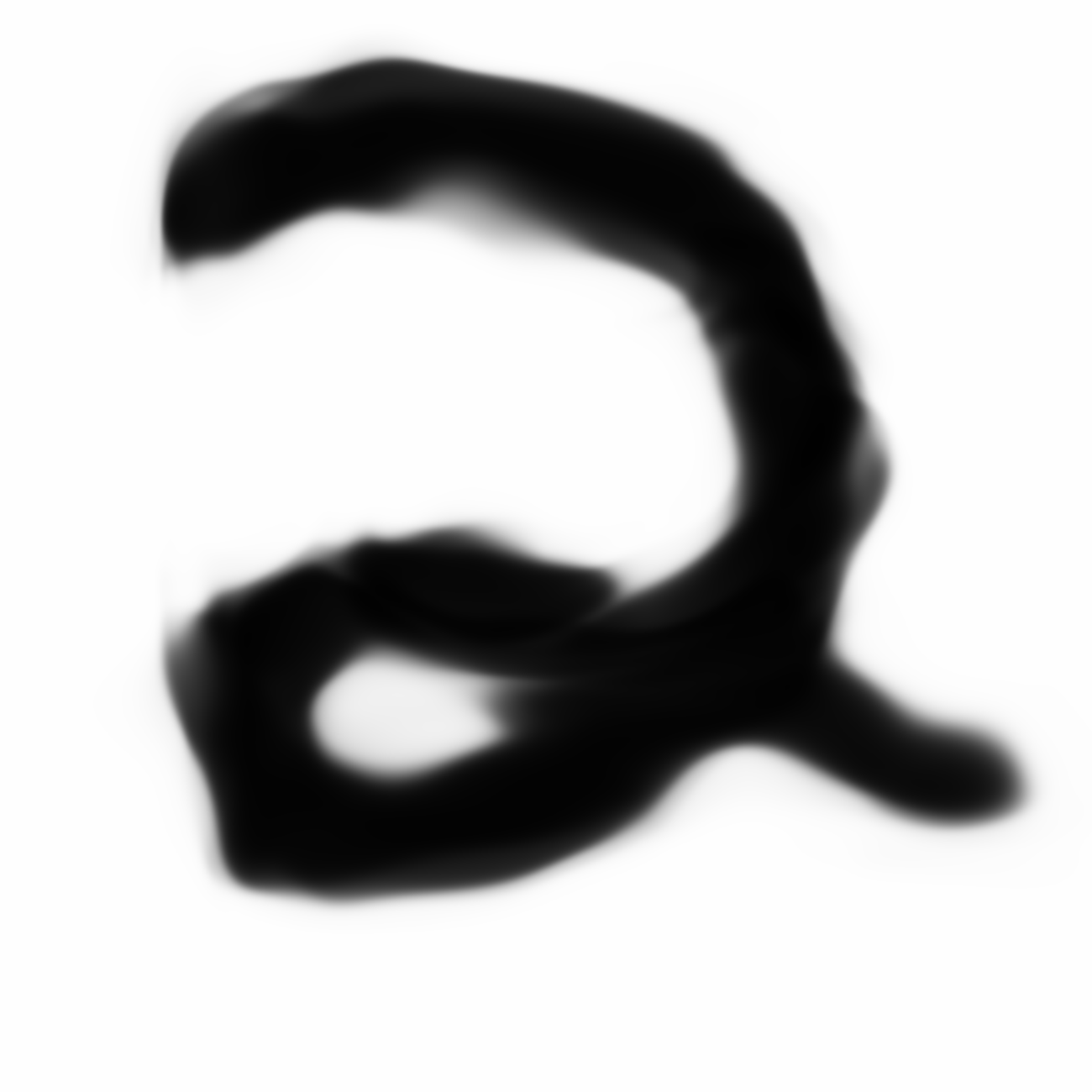
Same samples at much higher resolution:

|
|
|
Now we’re talking. I think these look kind of cool.
The much larger image that resembles zero looks a bit different than the other two larger images, and the reason was because the network that produced the image of zero was trained with a higher N_handicap value. Maybe this forces the generator network to overfit a bit during each batch and consequently the values of are pushed to levels that are a bit more extreme than they would otherwise have been if N_handicap were set lower. I kind of like this extra bit of punchiness as it adds character to the image when it gets blown up.
However, I find that in the end, the space of images generated from CPPN networks trained with this GAN method often get stuck and confined to two or three digits only. It was difficult to train a network that can generate all ten numerical digits. I think this is a weakness in the algorithm itself. There is nothing stopping G from finding its niche at generating a specific digit only, and be very good at generating that digit, so D still gets confused even if G only generates zeros.
We need to find a way to incorporate in our algorithm a penalty function that would penalise G if it couldn’t generate all the diverse examples, and in the next section I will talk about the Variational Encoder, which is a candidate to perform this penalty function. We will also merge the Variational Encoder with the Generative Adversarial Encoder, so that our network can generate MNIST digits that look real to actual MNIST images, are diverse enough to cover all ten digits, and be able to blow up the images to very high resolutions.
Combining Variational Encoder into the Model
To deal with the problem of generating a diverse set of examples, I combined a Variation Autoencoder (VAE) to our network. I am not going through the details of explaining VAE’s here, as there have been some great posts about them, and a very nice TensorFlow implementation.
VAE’s help use do two things. Firstly, they allow us to encode existing image into a much smaller latent Z vector, kind of like compression. It does this by passing an image through the encoder network, which we will call the Q network, with weights . And from this encoded latent vector Z, the generator network will produce an image that will be as close as possible to the original image passed in, hence it is an autoencoder system. This solves the problem we had in the GAN model, because if the generator only produces certain digits, but not other digits, it will get penalised as it is not reproducing many examples in the training set.
So far, we have assumed the Z vector to be simple independent unit gaussian variables. There’s no guarantee that the encoder network Q will encode images from a random training image X, to produce values of Z that belong to a probability distribution we can reproduce and draw randomly from, like a gaussian. Imagine we just stop here, and train this autoencoder as it is. We will lack the ability to generate random images, because we lack the ability to draw Z from a random distribution. If we draw Z from the gaussian distribution, it will only be by chance that Z will look like some value corresponding to the training set, and will produce images that do not look like the image set otherwise.
The ability to control the exact distribution of Z is the second thing the VAE will help us do, and the main why the VAE paper is such an important and influential paper. In addition to perform the autoencoding function, the latent Z variables generated from the Q network will also have the characteristic of being simple independent unit gaussian random variables. In other words, if X is a random image from our training set, belonging to whatever weird and complicated probability distribution, the Q network will make sure the Z is constructed in a way so that P(Z|X) is a simple set of independent unit gaussian random variables. And the amazing thing is, this difference between the distribution of P(Z|X) and the distribution of a gaussian distribution (they call this the KL Divergence) can be quantified and minimised using gradient descent using some elegant mathematical machinery, by injecting gaussian noise into the output layer of the Q network. This VAE model can be trained by minimising the sum of both the reconstruction error and KL divergence error using gradient descent, in Equation 10 of the VAE paper.
Our final CPPN model combined with GAN + VAE:

|
Rather than sticking with the pure VAE model, I wanted to combine VAE with GAN, because I found that if I stuck with only VAE, the images it generated in the end looked very blurry and uninteresting when we blow up the image. I think this is due to the error term being calculated off pixel errors, and this is a known problem for the VAE model. Nonetheless, it is still useful for our cause, and if we are able to combine it with GAN, we may be able to train a model that will be able to reproduce every digit, and look more realistic with the discriminator network acting as a final filter.
Training this combined model will require some tweaks to our existing algorithm, because we will also need to train to optimise the VAE’s error. Note that we will adjust both and when optimising for both G_loss and VAE_loss.
CPPN+GAN+VAE algorithm for 1 epoch of training:
1
2
3
4
5
6
7
8
9
10
11
12
13
14
15
16
17
18
19
20
21
22
23
24
25
26
27
28
29
30
31
32
Randomise Sample Images in Training Set
For each Sample Image in Training Set
y_real = Discriminator(Sample Image, w_d)
# Q Network Optimisation
For i: 1 .. 4
Z_vae_noise = Normal(mean = 0, stdev = 1, Size=(1, N_z))
Z = Encoder(Sample Image, Z_vae_noise)
Image = Generator(Z, w_g)
Calculate VAE_loss = Reconstruction Loss + KL Divergence Loss
Calculate dVAE_loss/dW_q and dVAE_loss/dW_g gradients via backprop
Adjust W_q's and W_g's using SGD-type optimising step
# D Network Optimisation
For i: 1 .. 4
Z_vae_noise = Normal(mean = 0, stdev = 1, Size=(1, N_z))
Z = Encoder(Sample Image, Z_vae_noise)
Image = Generator(Z, w_g)
y_fake = Discriminator(Image, w_d)
Calculate G_loss
Calculate dG_loss/dW_g and dG_loss/dW_q gradients via backprop
#i.e., the direction that would make D crappier
Adjust W_g's W_q's using SGD-type optimising step
# Optimise D Network only if it is not that far ahead.
Calculate D_loss
if G_loss < th_high and D_loss > th_low
Calculate dD_loss/dW_d via backprop
#i.e., the direction that would make D better
Adjust W_d's using SGD-type optimising step
The trick here, is to structure and balance all the subnetworks’ structure, so that G_loss and D_loss hovers around 0.69, so they are mutually trying to improve by fighting each other over time, and improve at the same rate. In addition, we should see the VAE_loss decrease over time epoch by epoch, while the other two networks battle out each other. It is kind of a black art to train these things, and maintain balance. The VAE is trying to walk across a plank connecting two speed boats (G and D) trying to outrace each other.
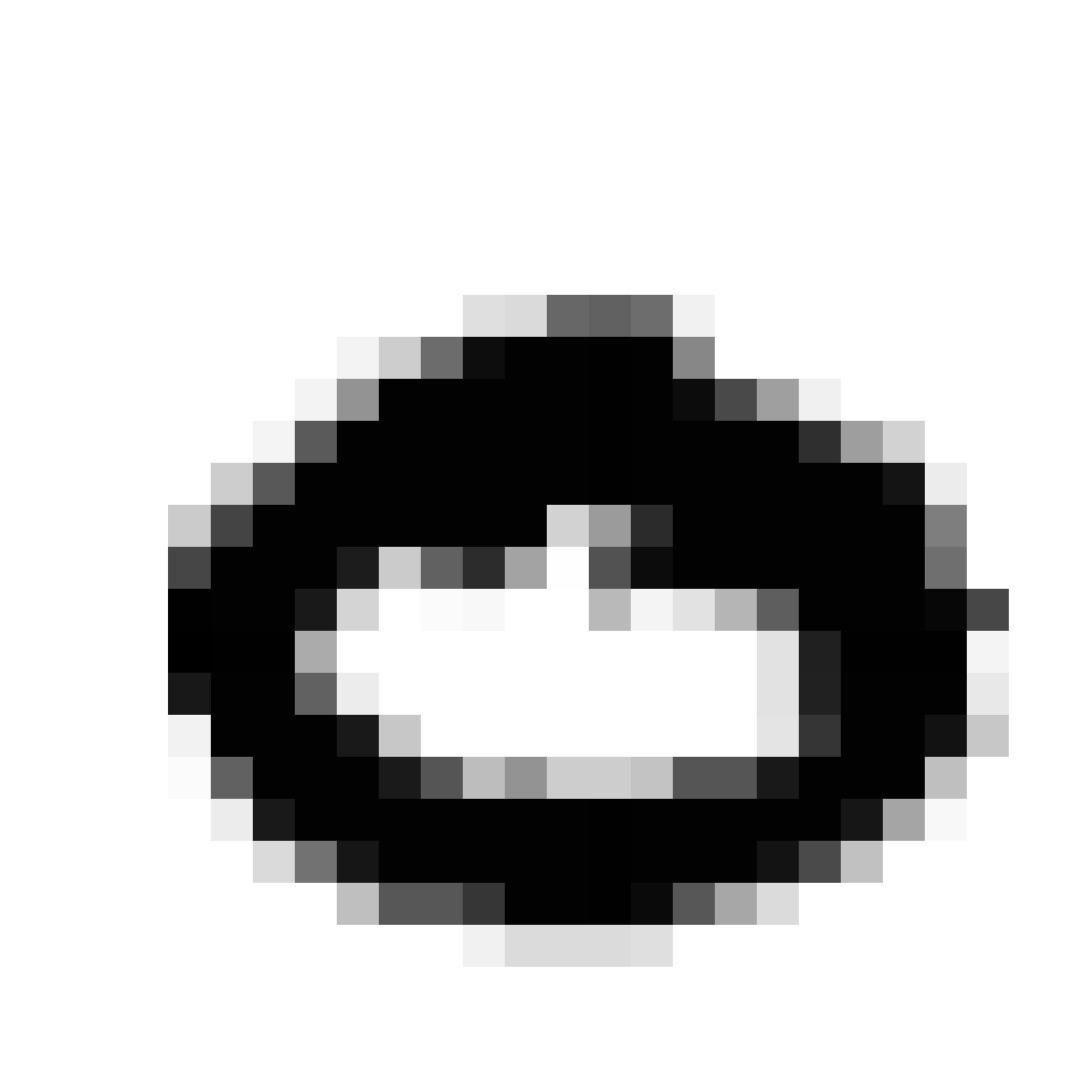
After training the model, we can see the results of feeding random vectors of Z, drawn from unit gaussian distribution, into our G network, and we can generate some random large images. Let’s see what we end up with!
Random latent vectors
We can generate some random large samples from our trained model in IPython:
1
2
3
4
5
%run -i sampler.py
sampler = Sampler()
z = sampler.generate_z() # vector of 32 random gaussian samples ~ N(0, 1)
x = sampler.generate(z) # from z, generate an image x, which is a np.array
sampler.show_image(x) # display this image interactively in IPython
|
|
|
|
|
|
|
|
|
We can see how our generator network takes in any random vector Z, consisting of 32 real numbers, and generates a random image that sort of looks like a number digit based on the values of Z.
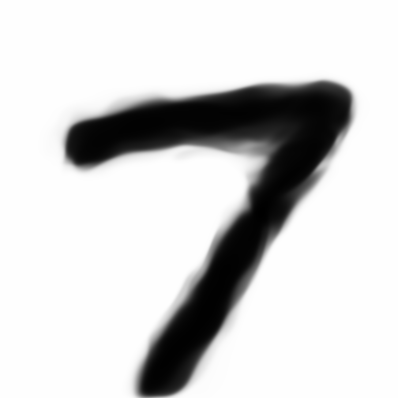
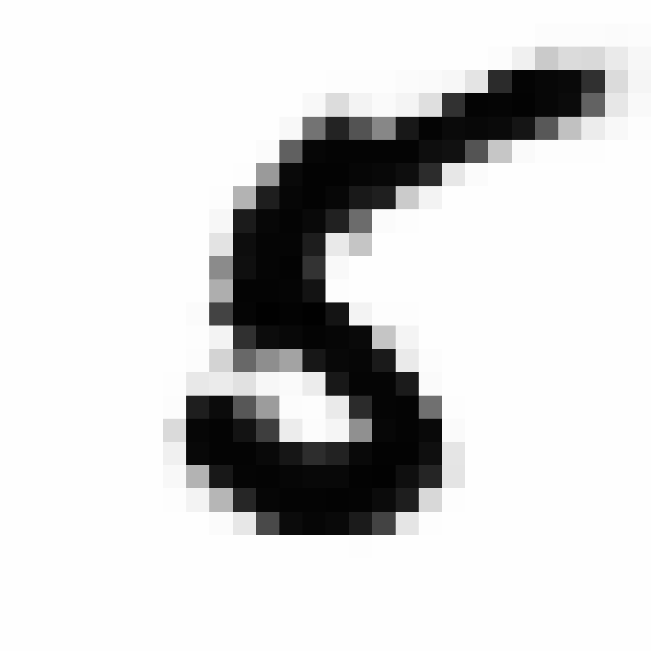
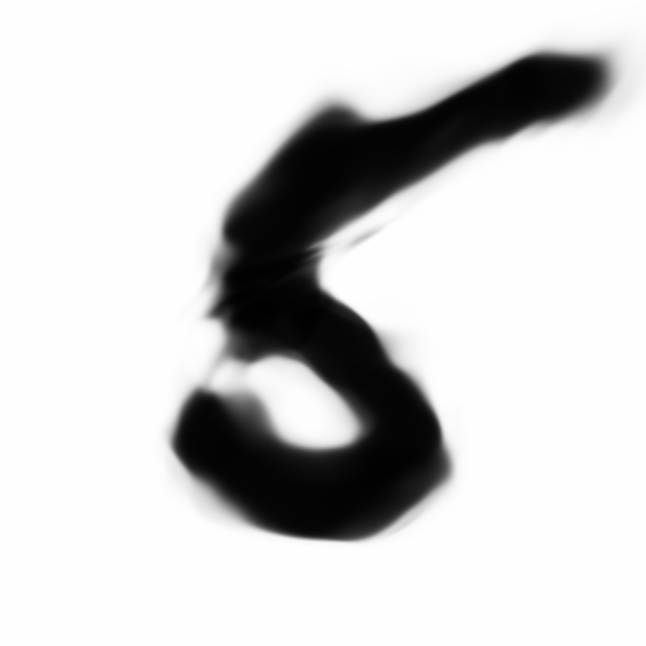
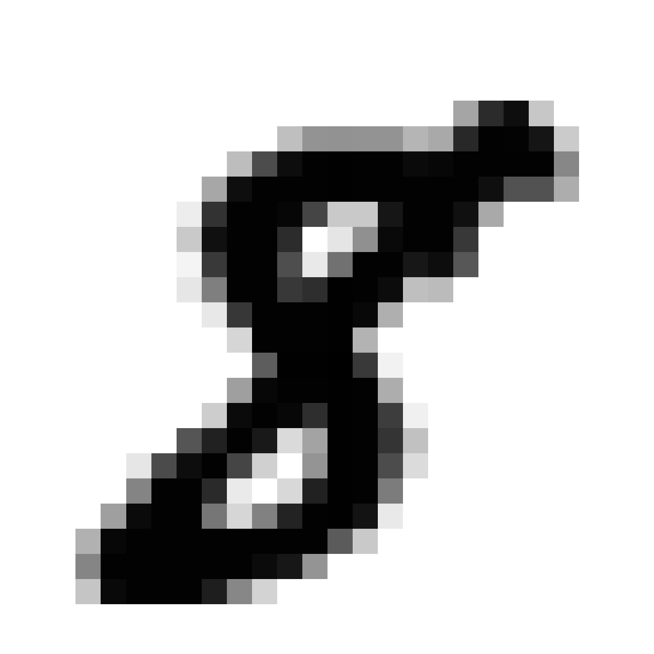
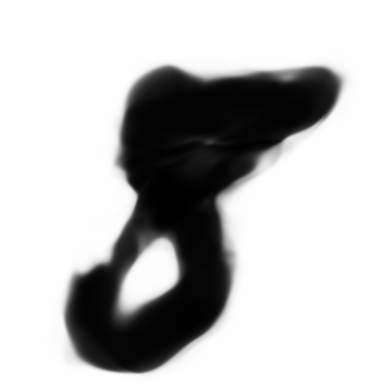
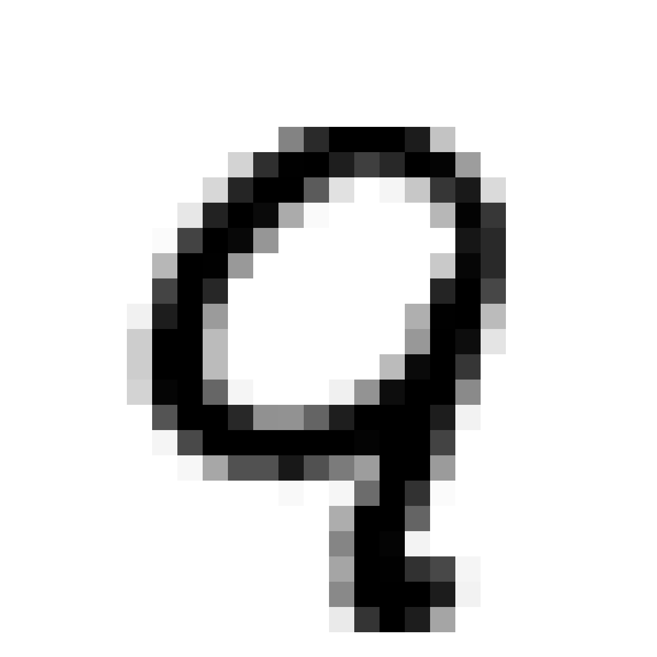
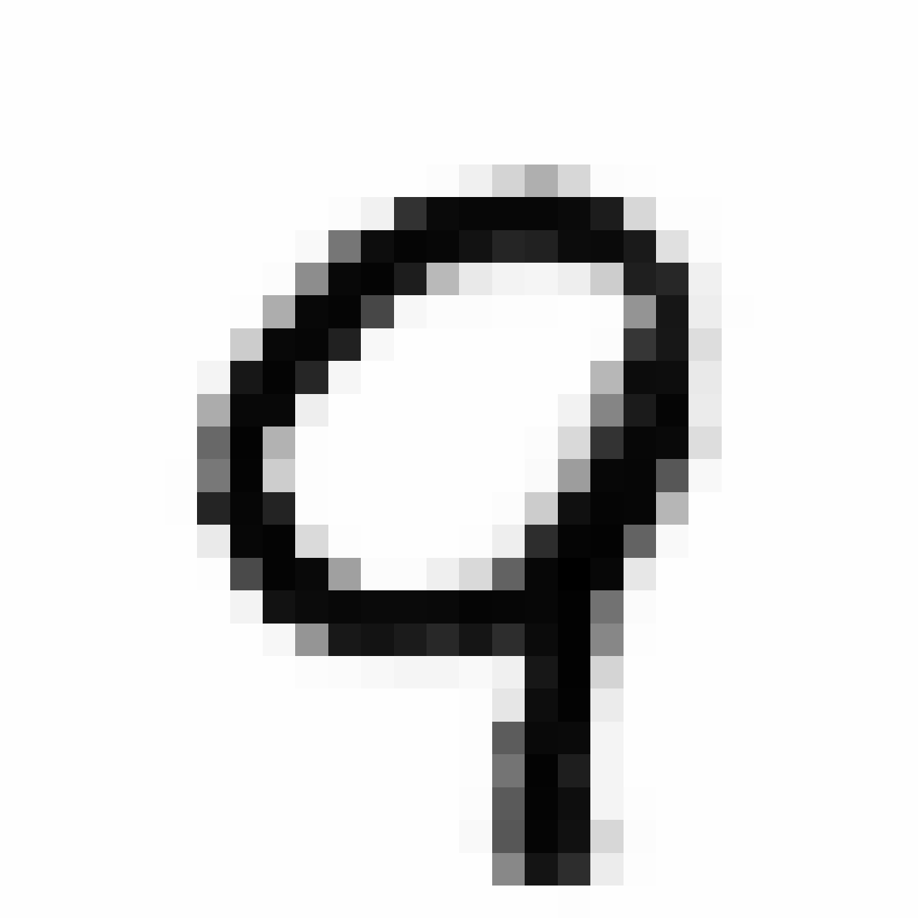
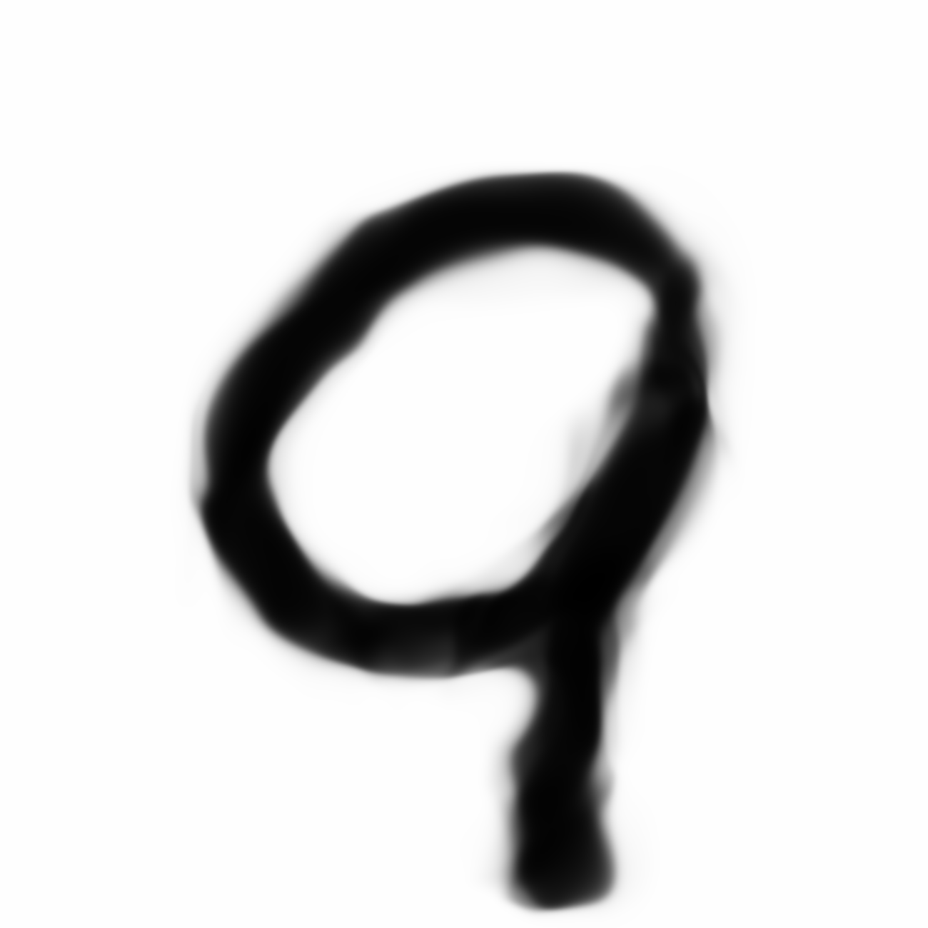
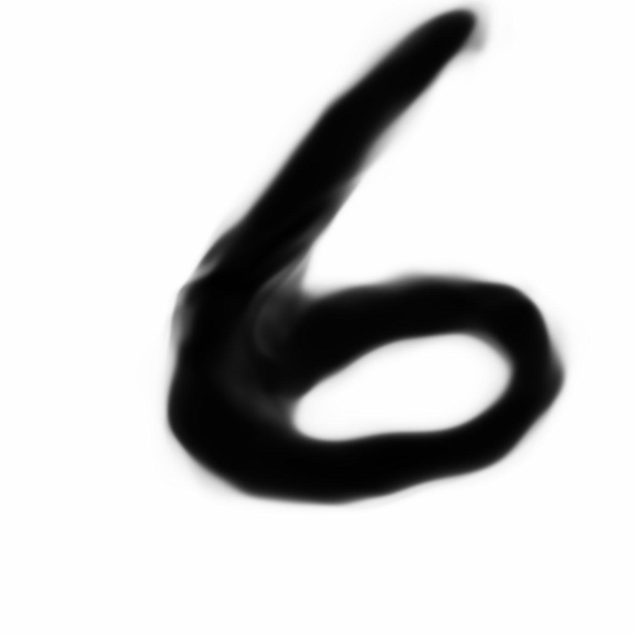
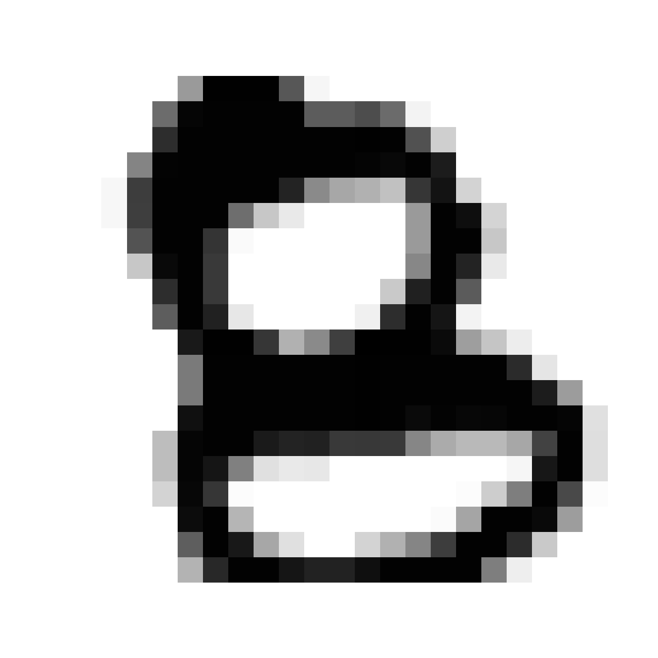
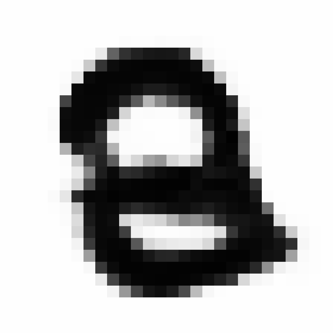
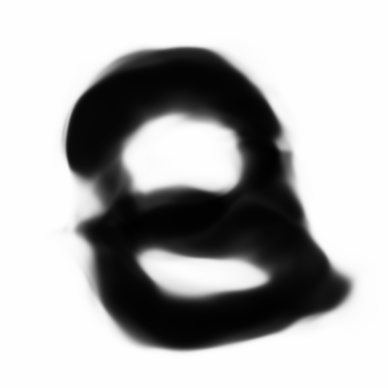
The next thing we want to try is to compare actual MNIST examples to the autoencoded ones. That is, take a random MNIST image, encode the image to a latent vector Z, and then generate back the image. We will first generate the image with the same dimensions as the example (26x26), and then an image 50 times larger (1300x1300) to see the network imagine what MNIST should look like were it much larger.
First, we draw a random picture from MNIST and display it.
1
2
m = sampler.get_random_mnist() # get a random image from the mnist dataset
sampler.show_image(m) # show the raw mnist sample in IPython
Then, we encode that picture into Z.
1
z = sampler.encode(m) # encode the picture to a latent vector
From Z, we generate a 26x26 reconstruction image.
1
2
x_26x26 = sampler.generate(z, x_dim = 26, y_dim = 26)
sampler.show_image(x_26x26)
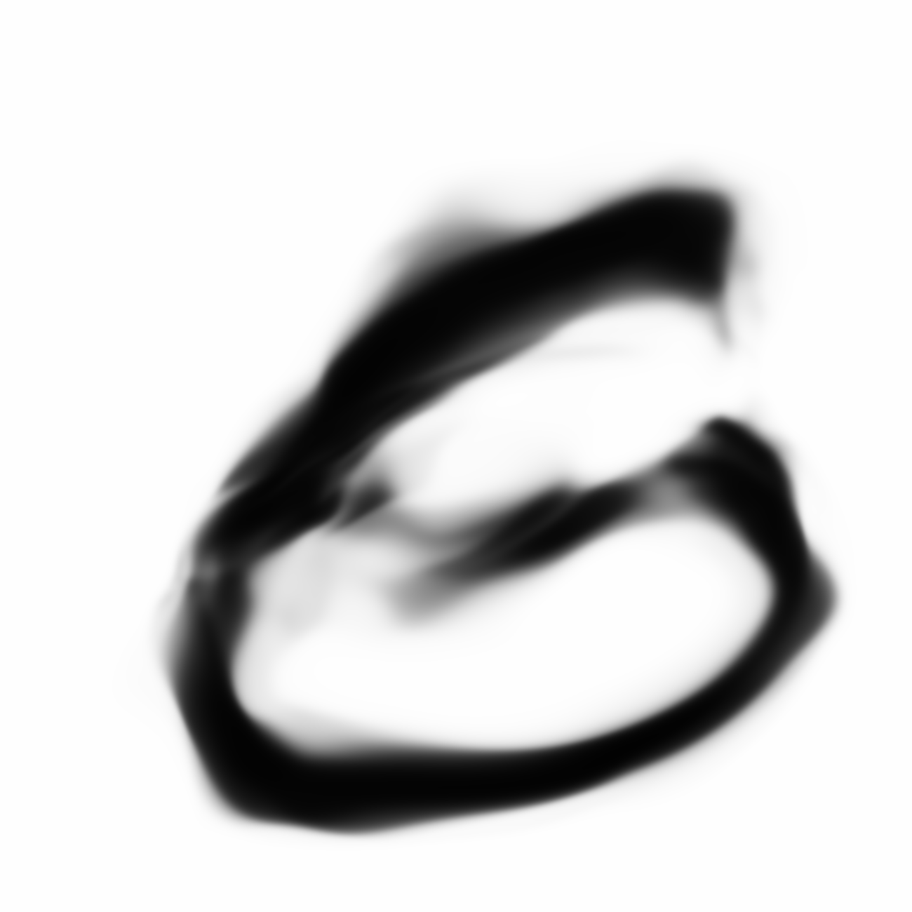
We can also generate much larger reconstruction image using the same Z.
1
2
x_1300x1300 = sampler.generate(z, x_dim = 1300, y_dim = 1300)
sampler.show_image(x_1300x1300)
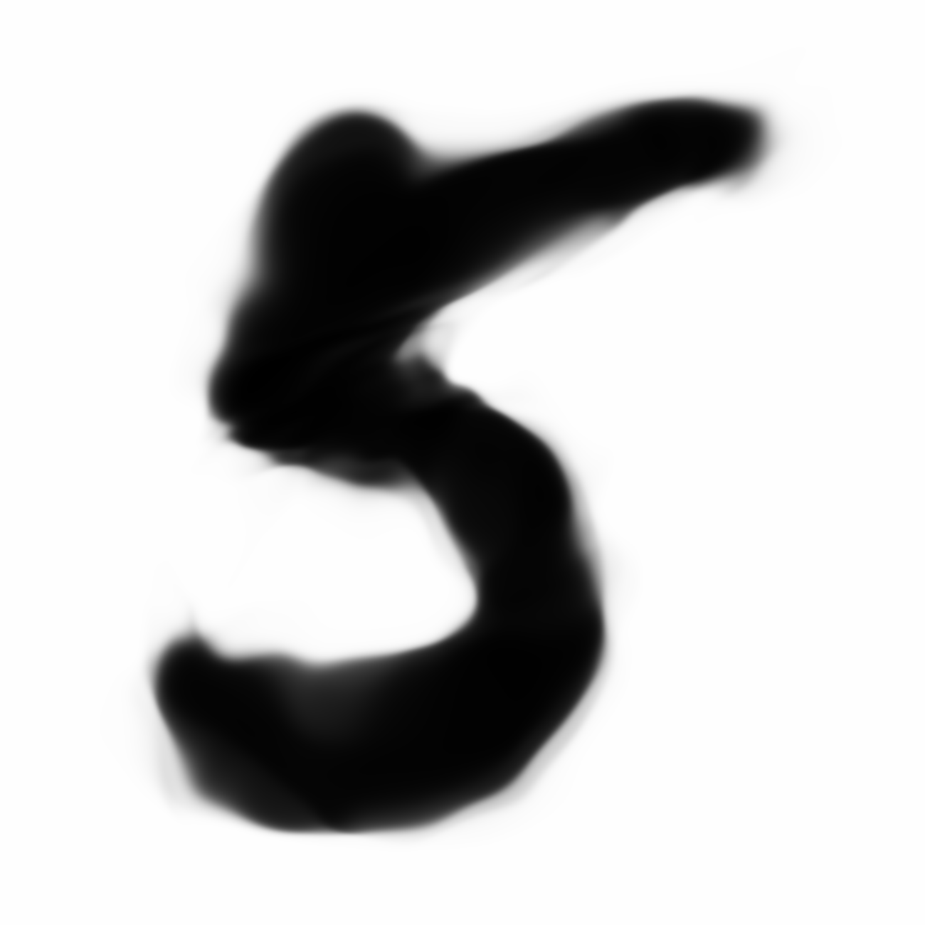
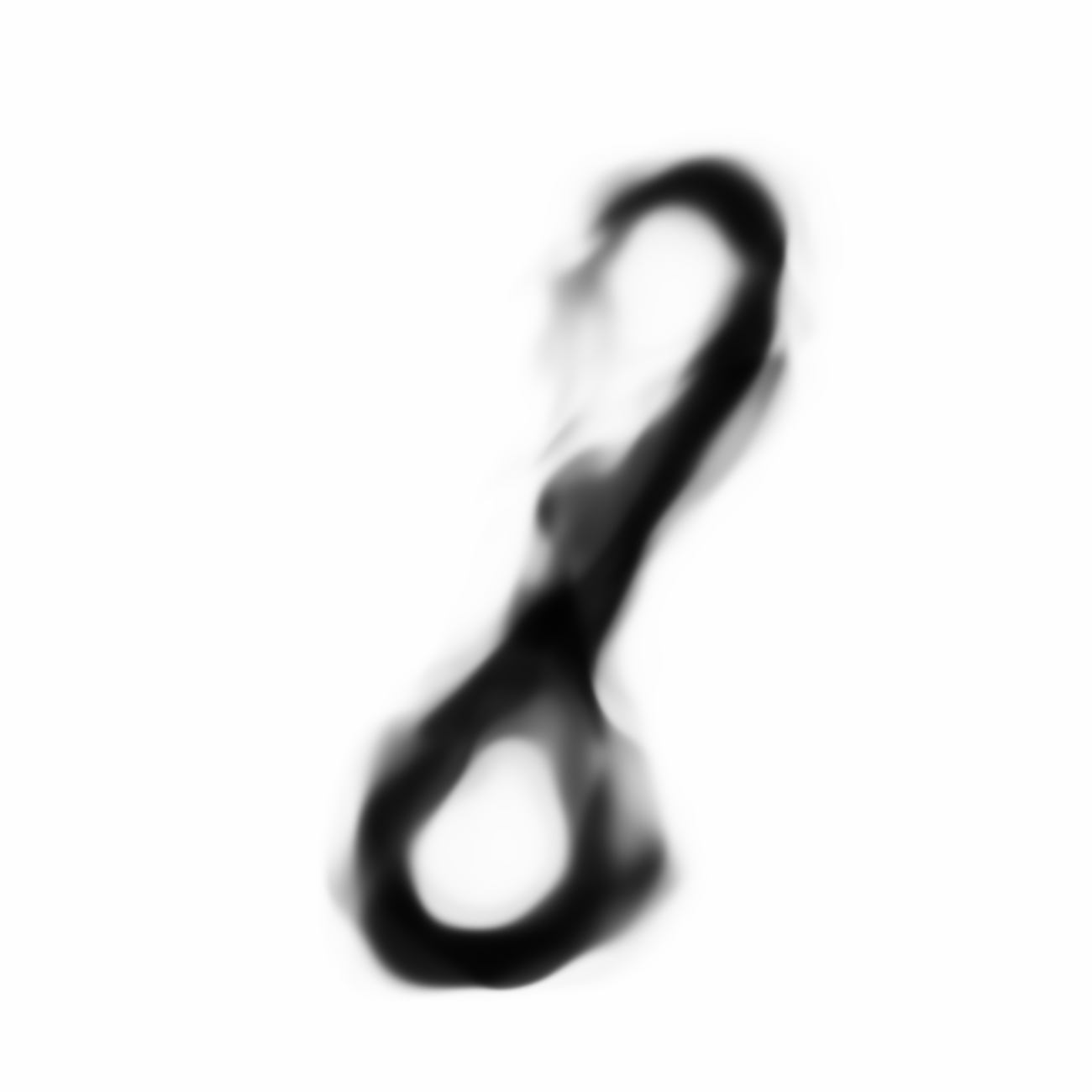
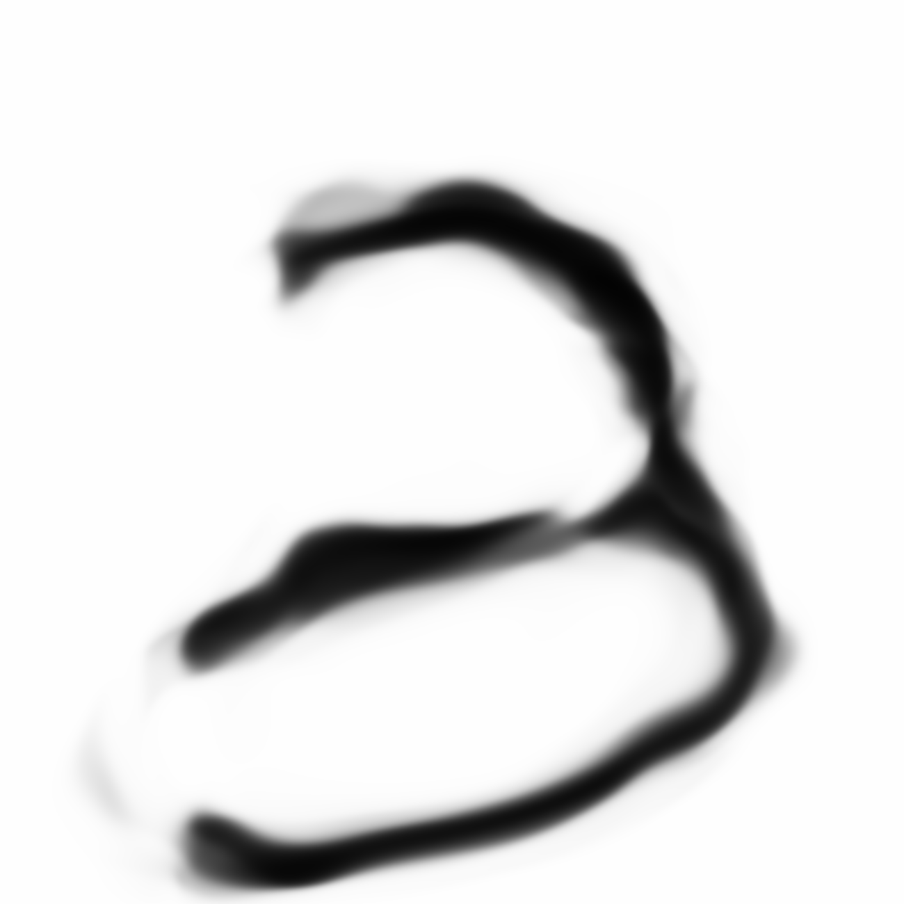
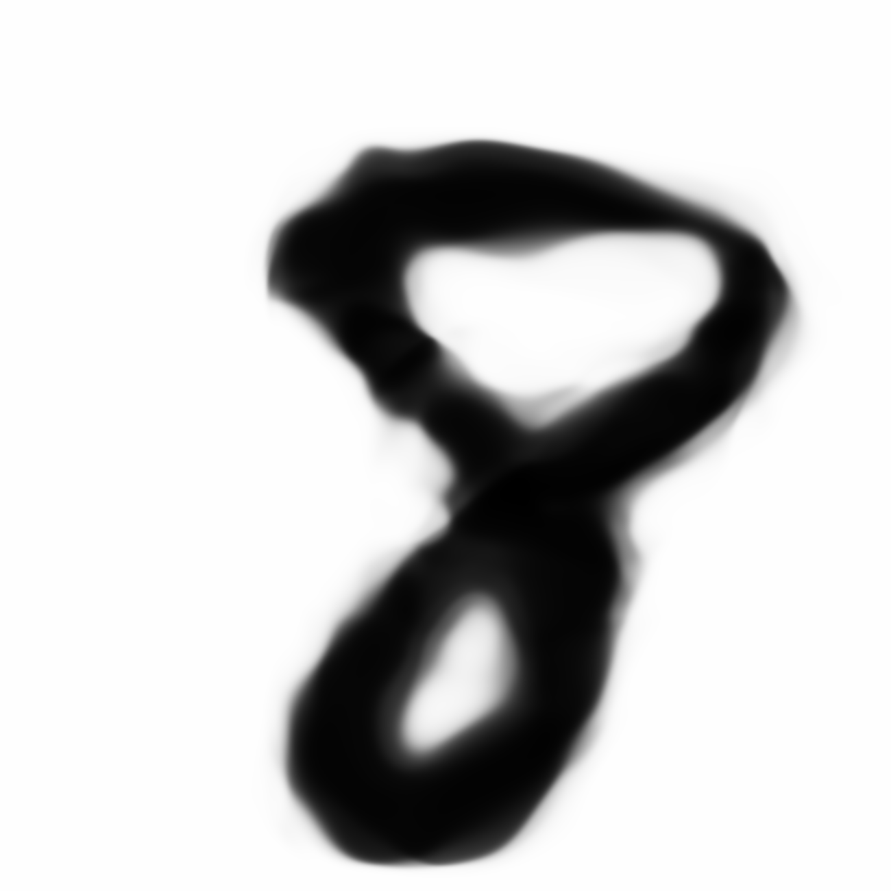
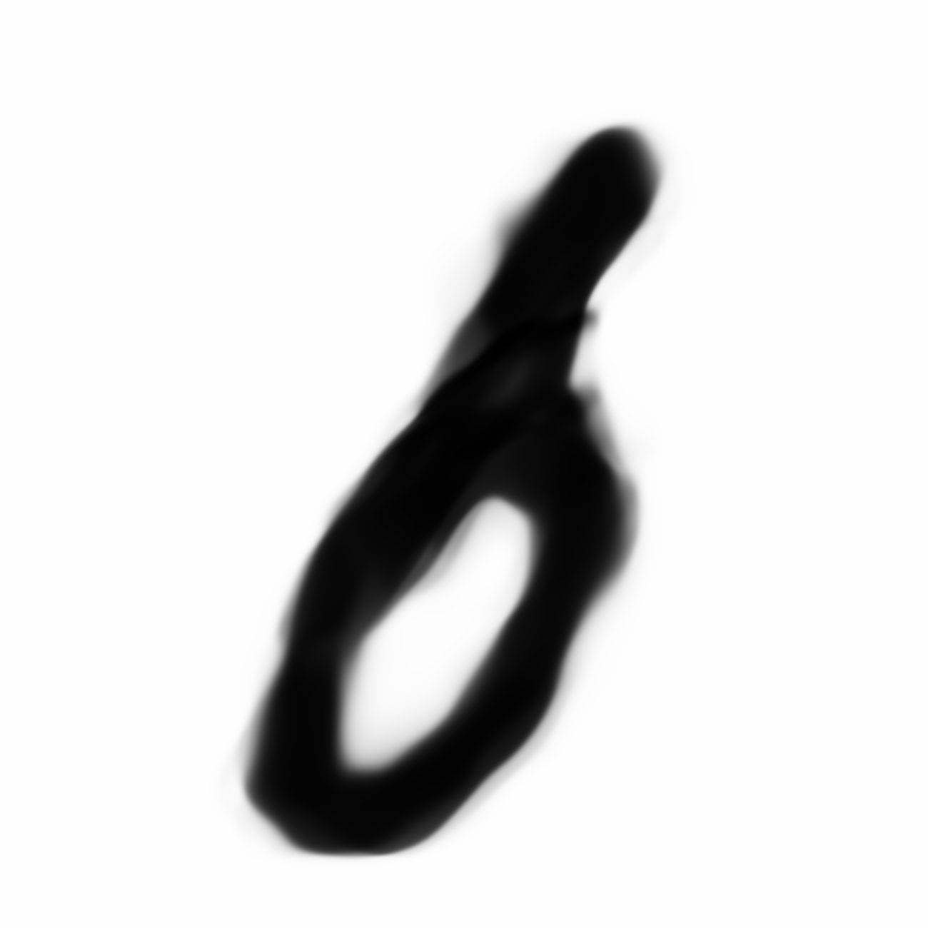
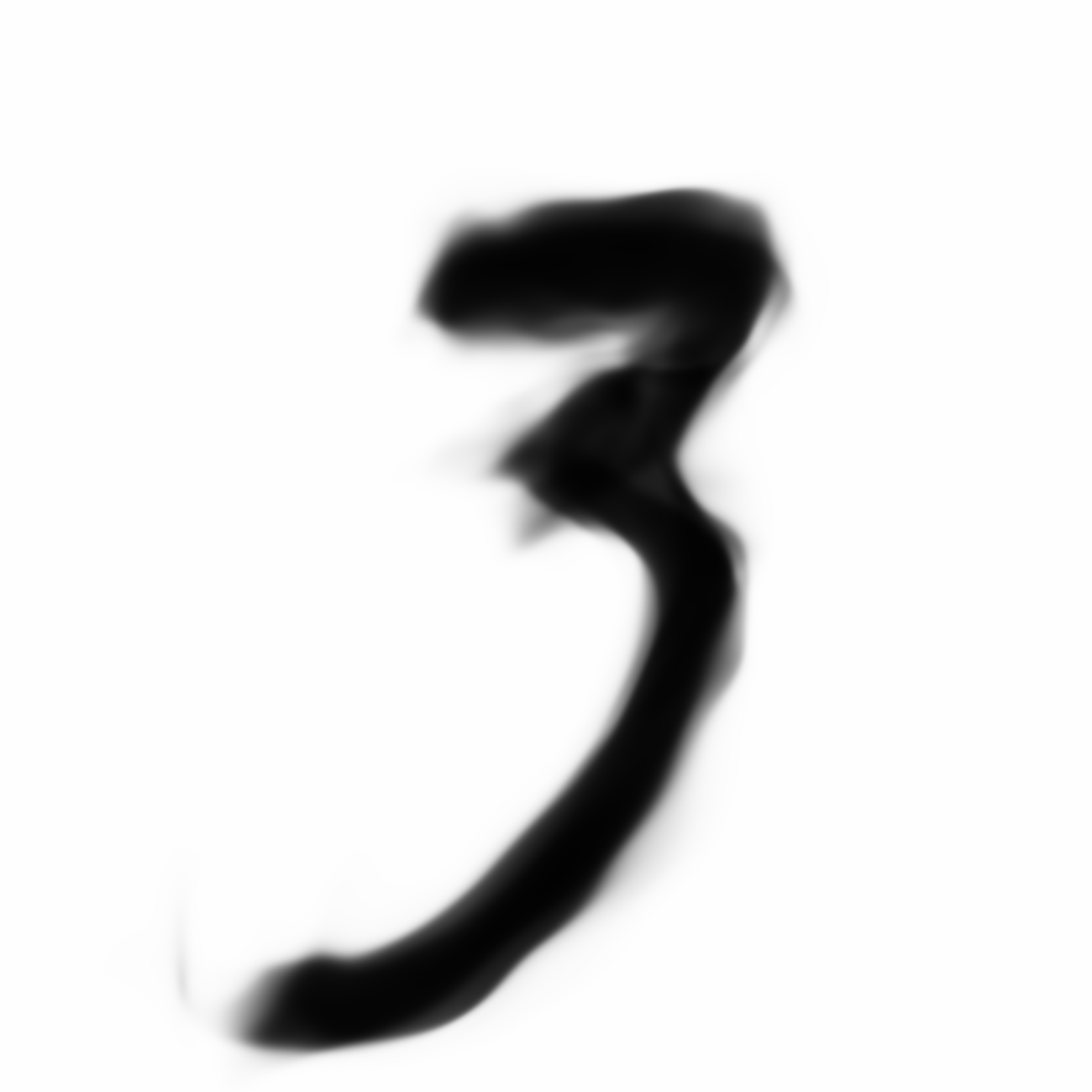
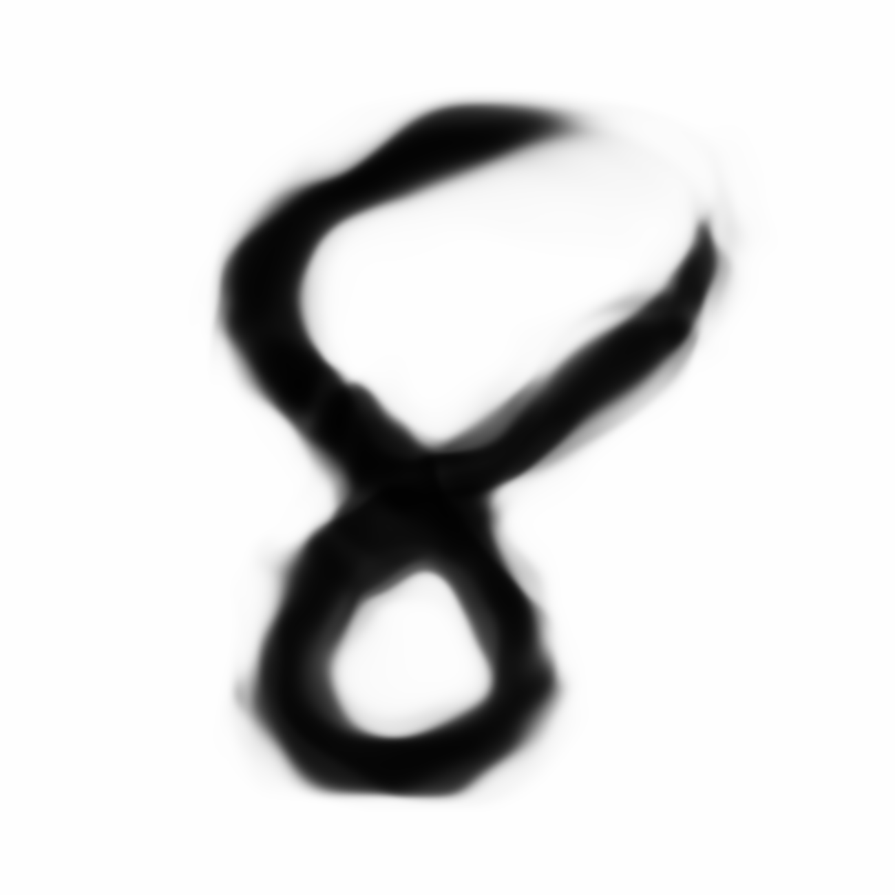
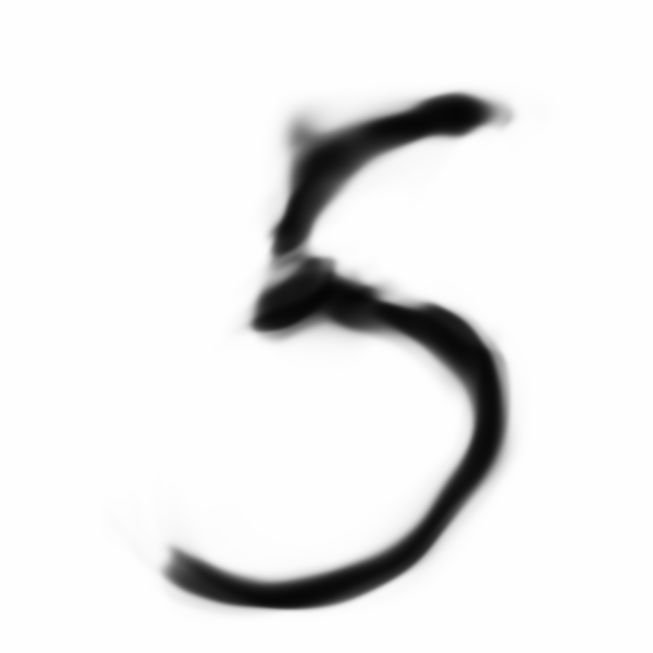
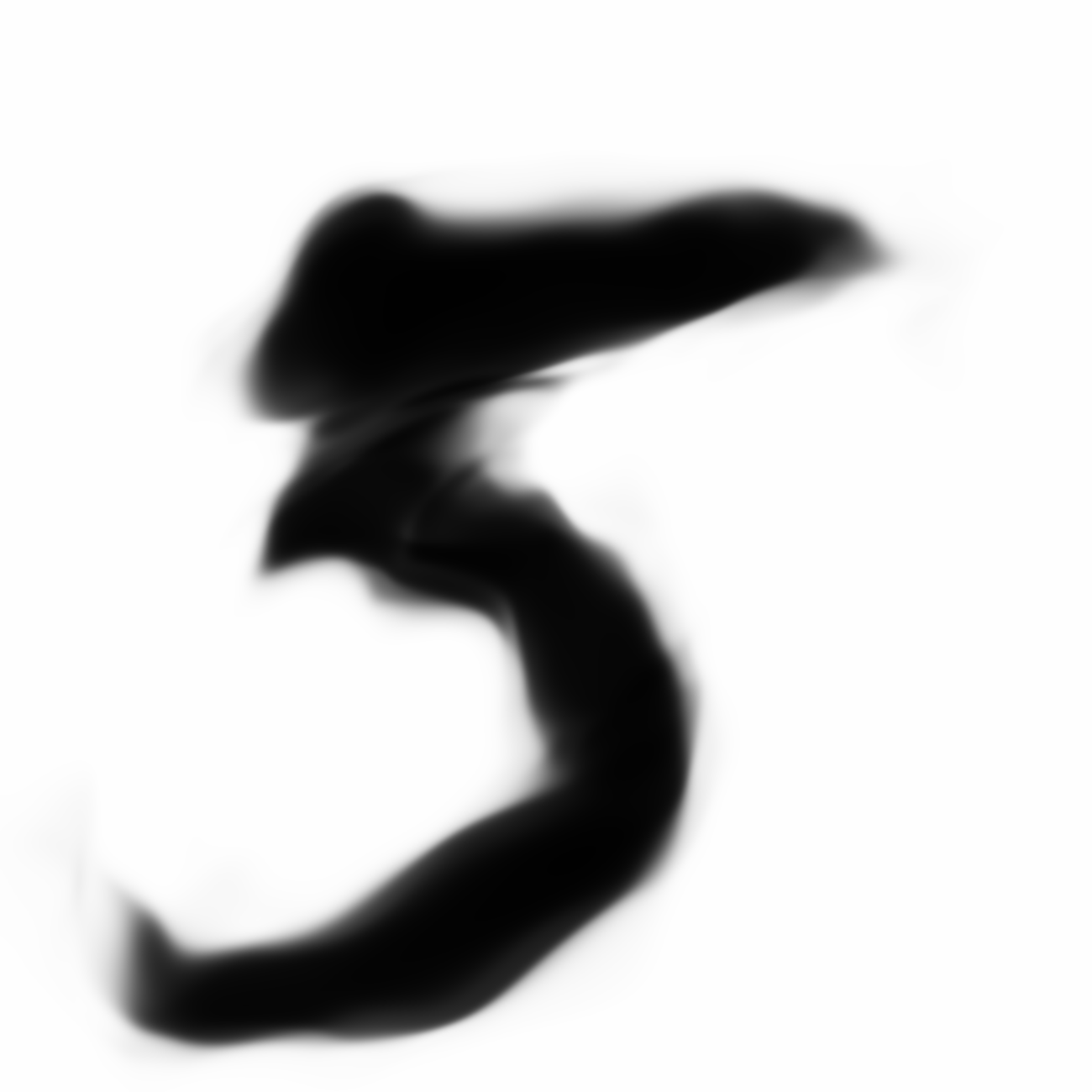
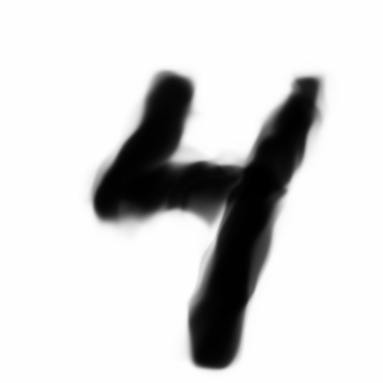
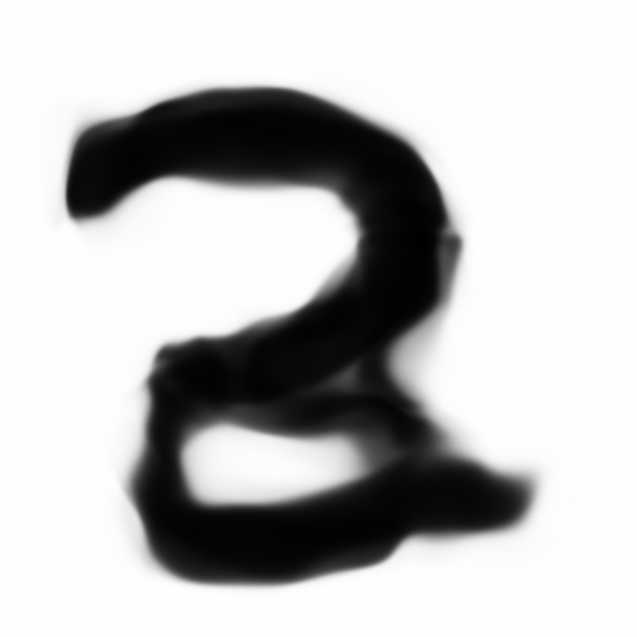
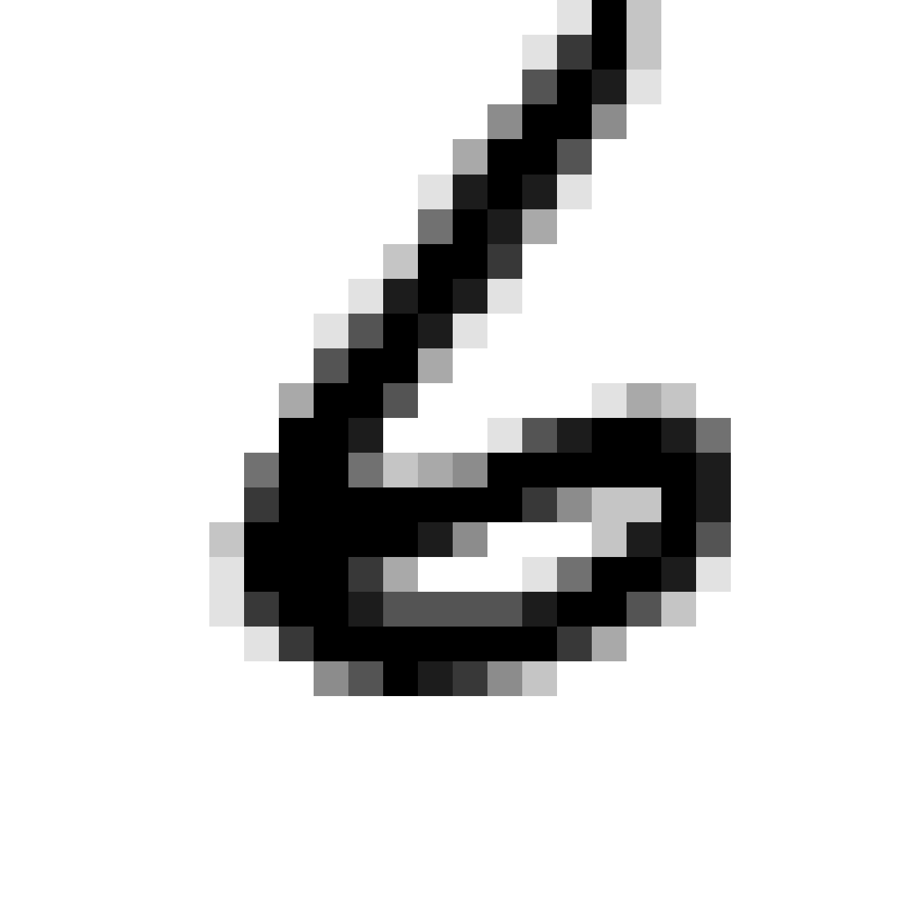
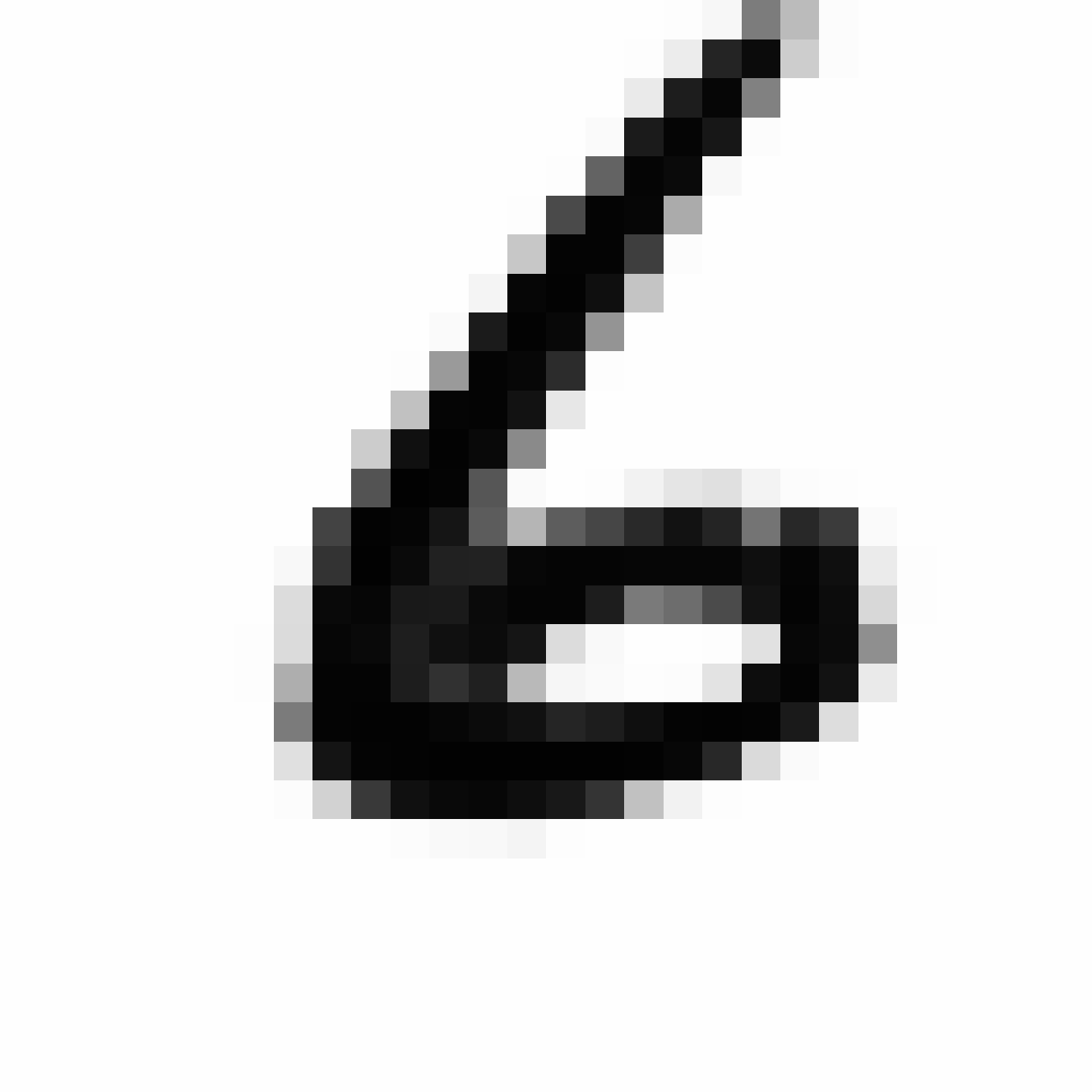
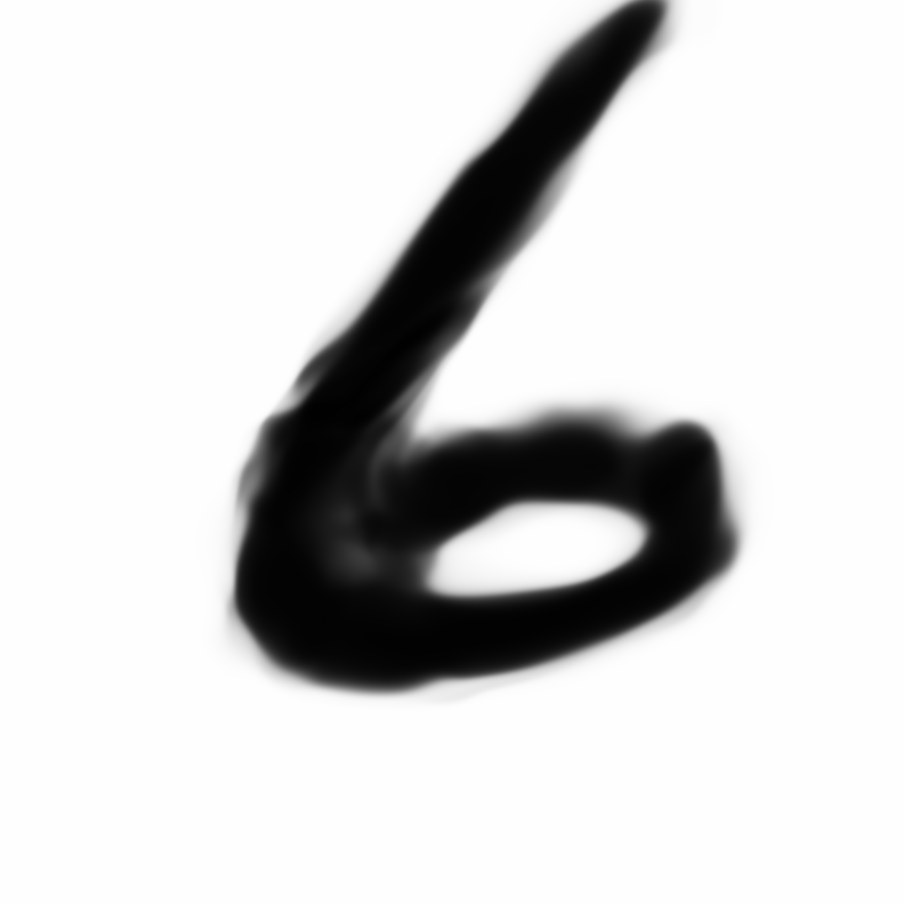
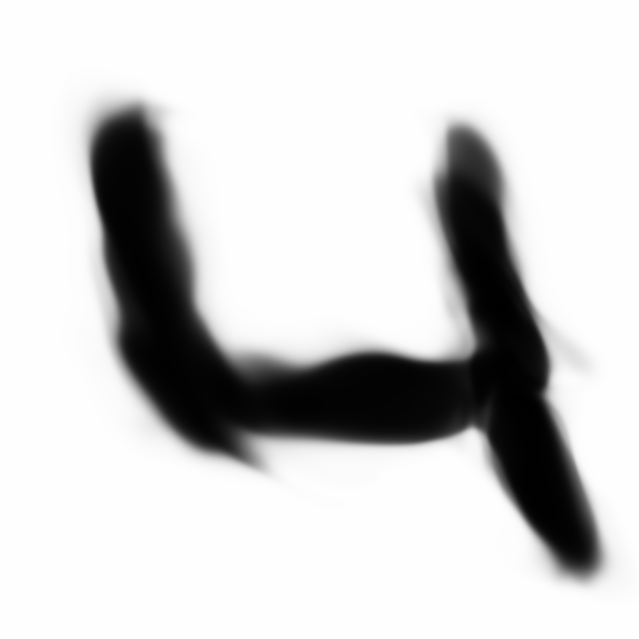
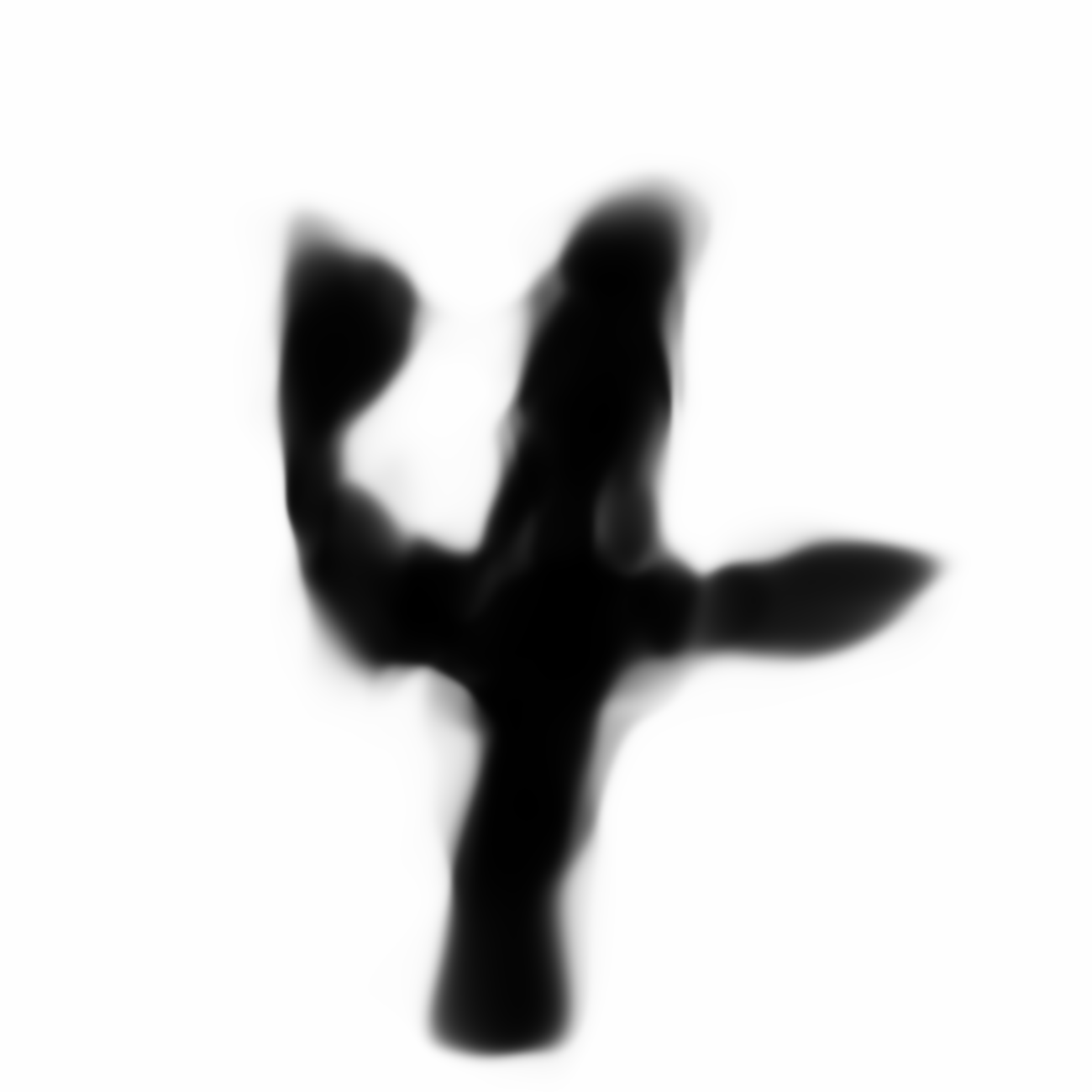
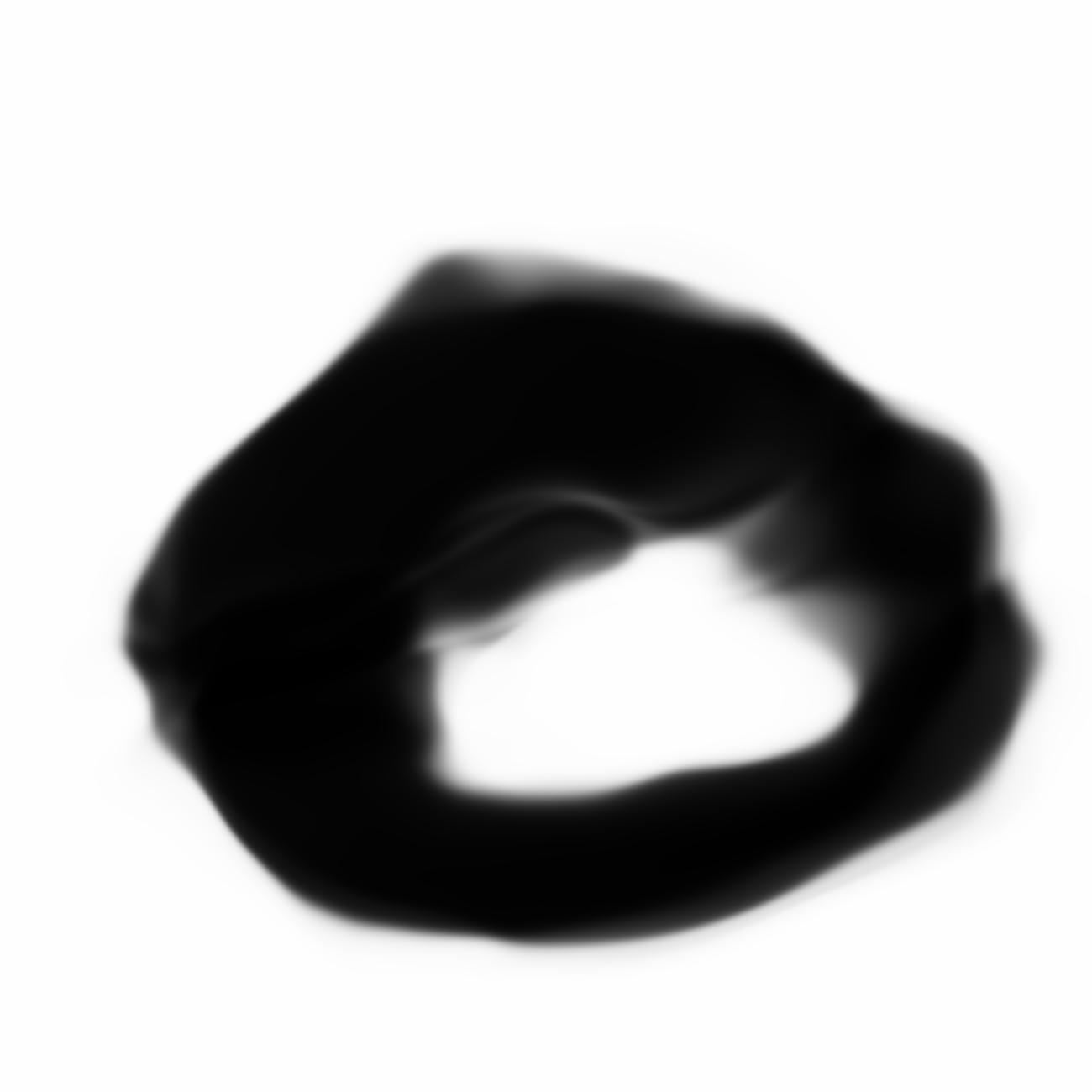
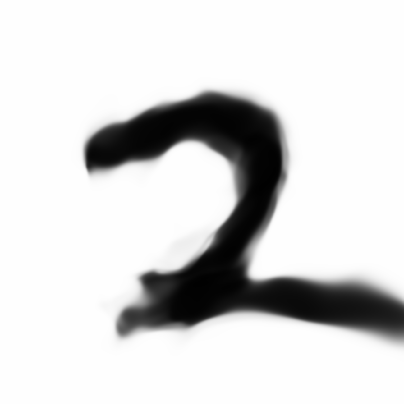
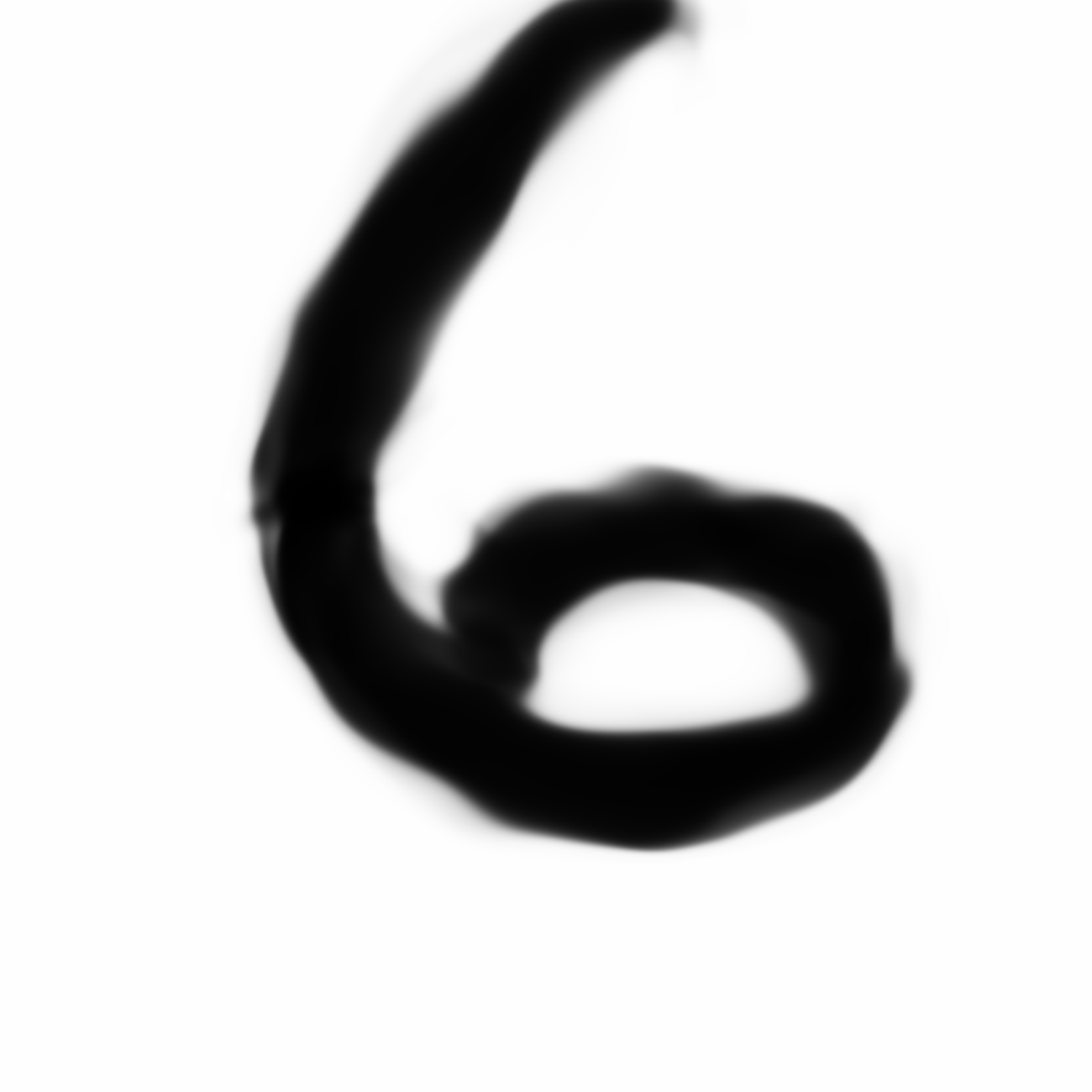
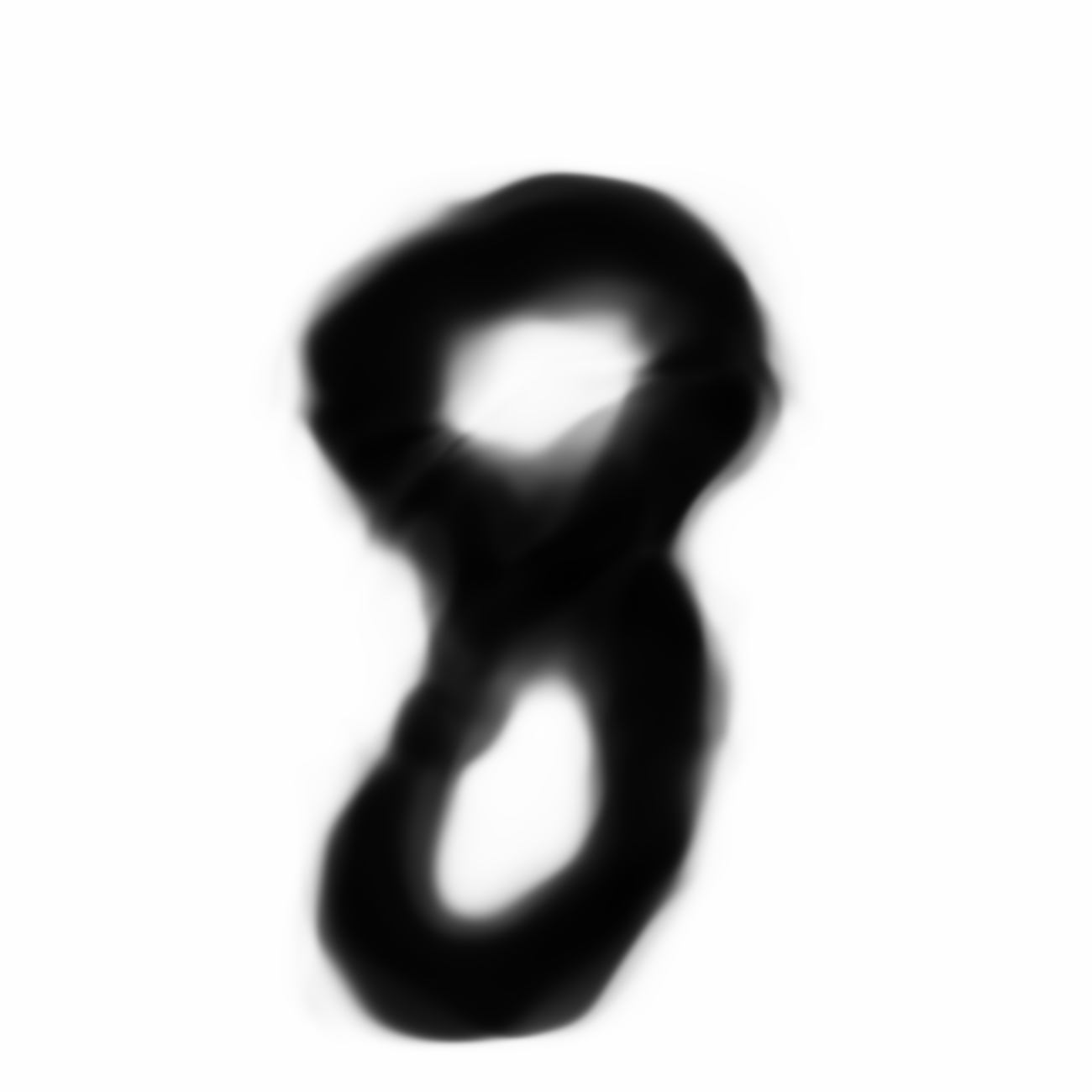
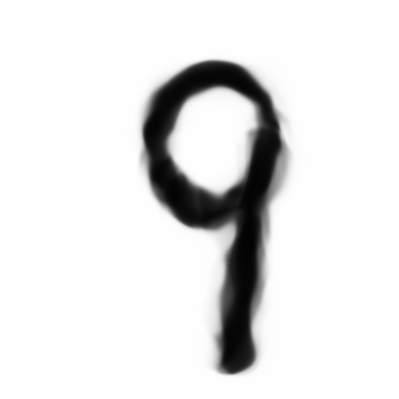
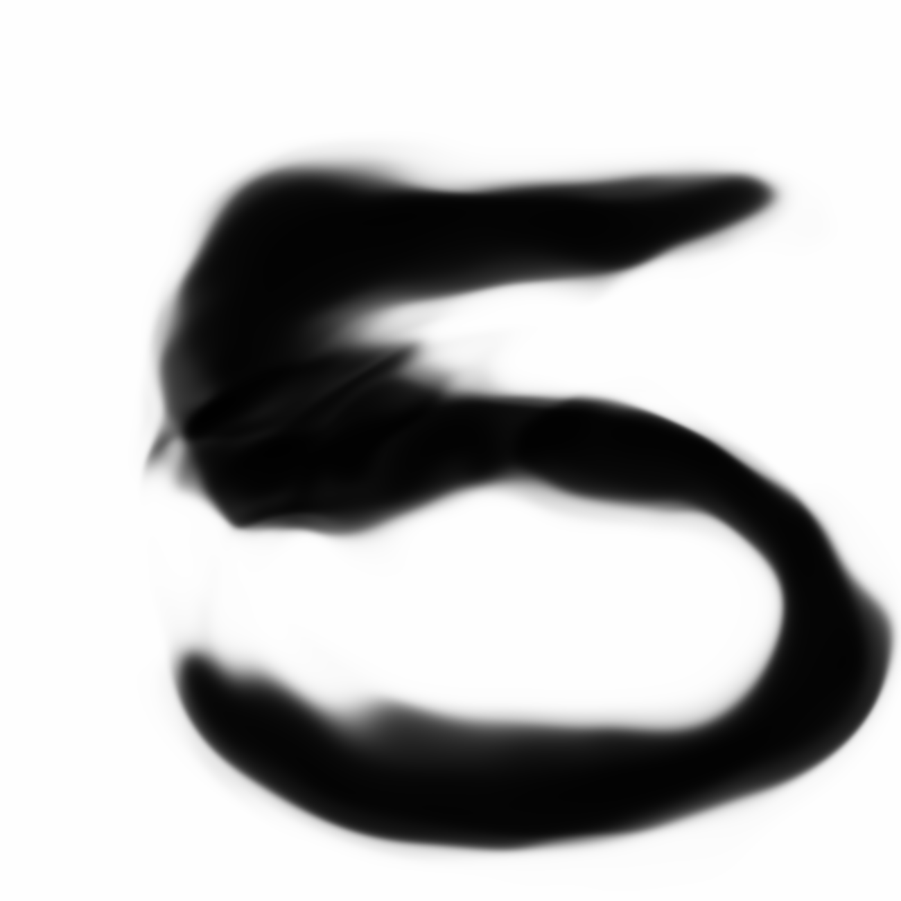
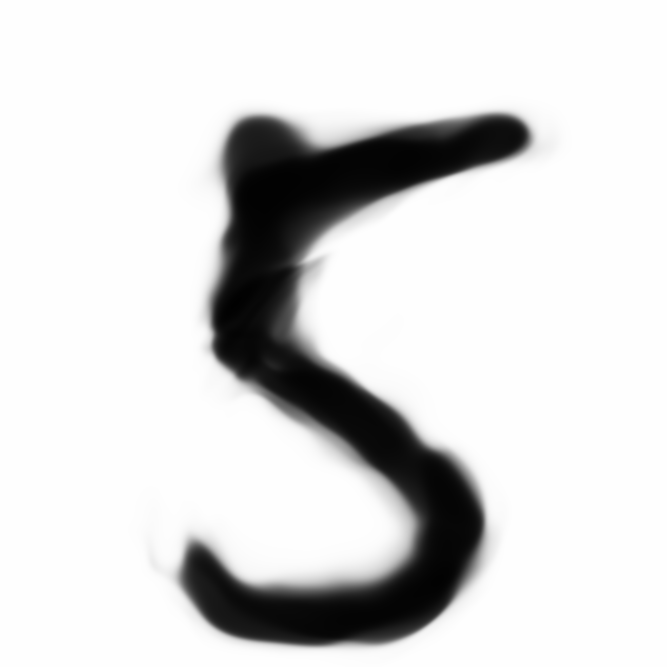
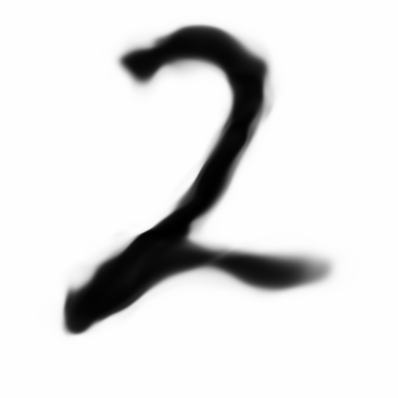
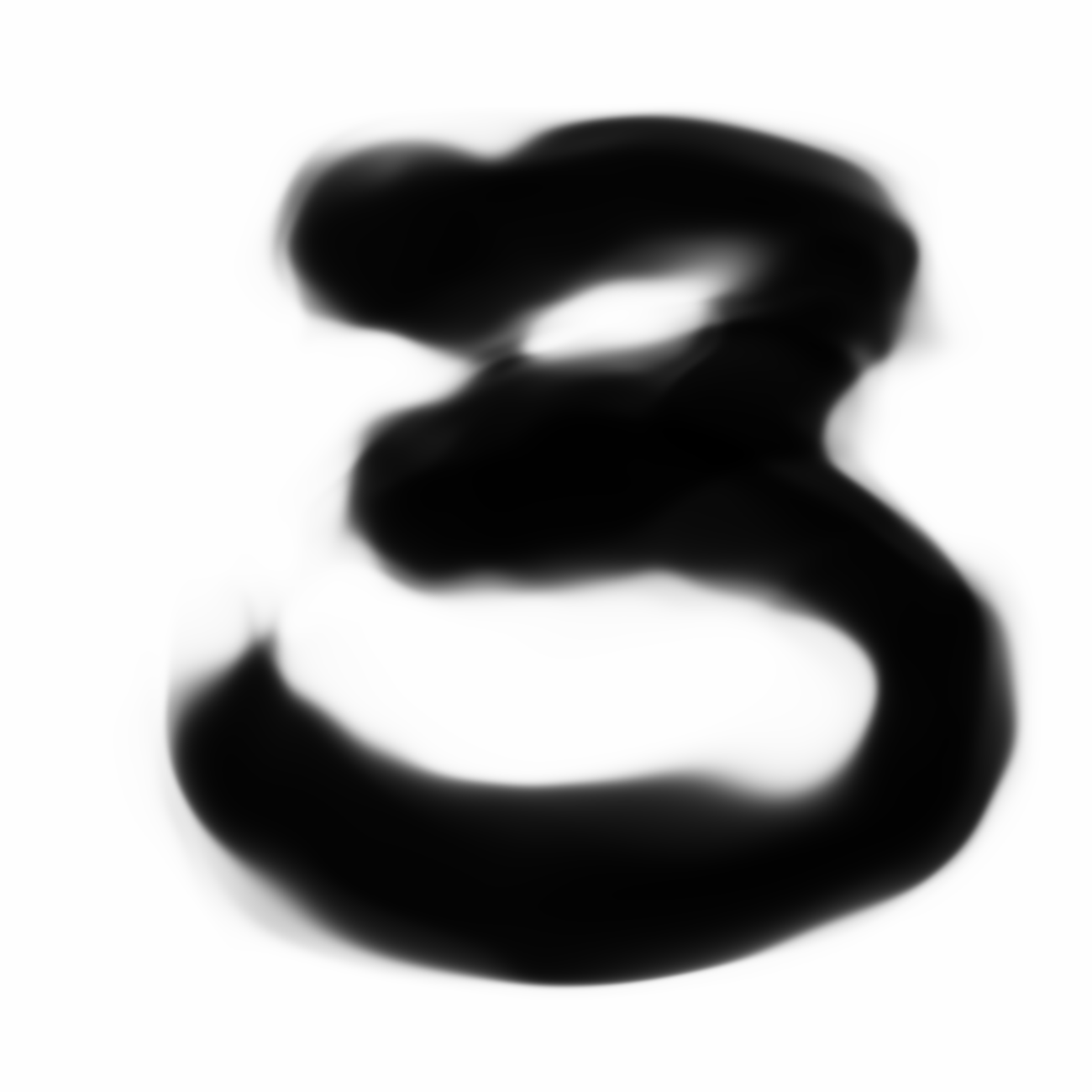
The current VAE+GAN structure seems to produce cloudy versions of MNIST image when we scale them up, like trying to draw something from smoke.
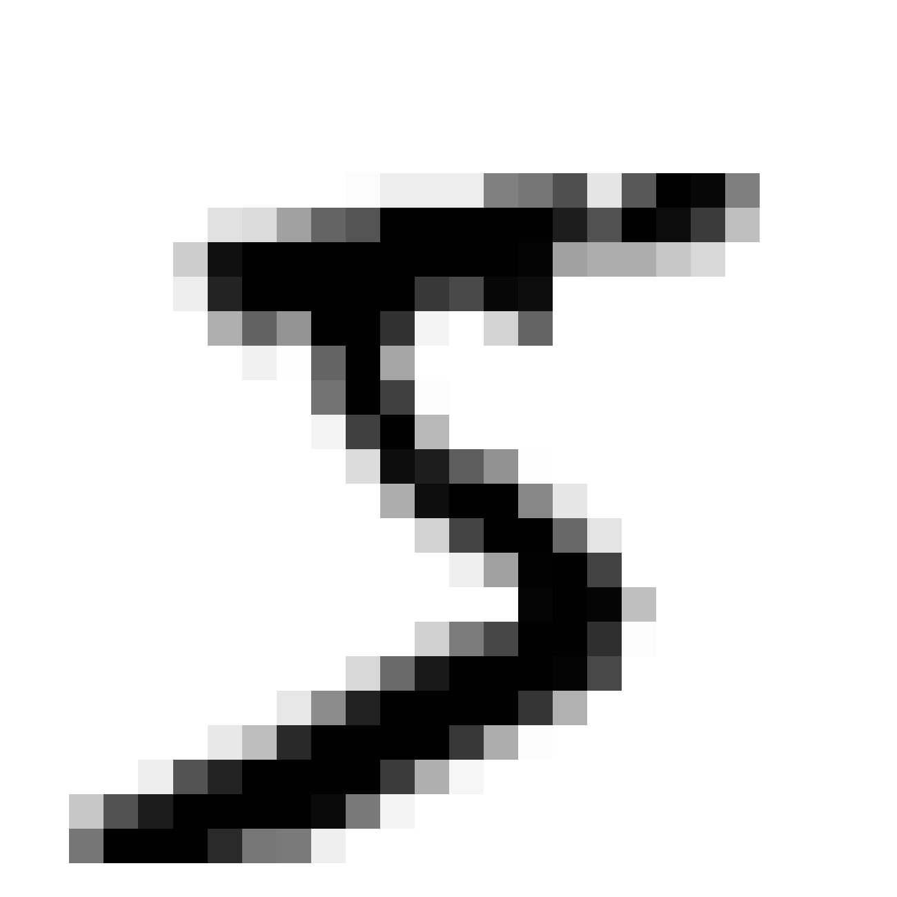
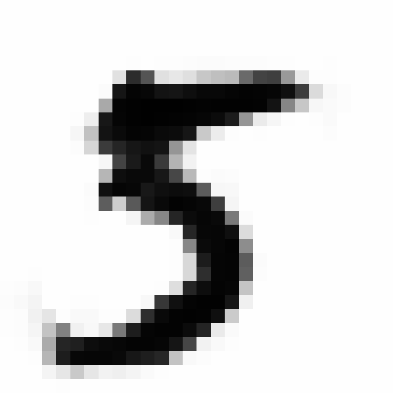
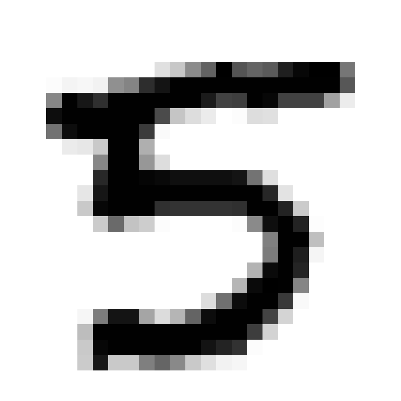
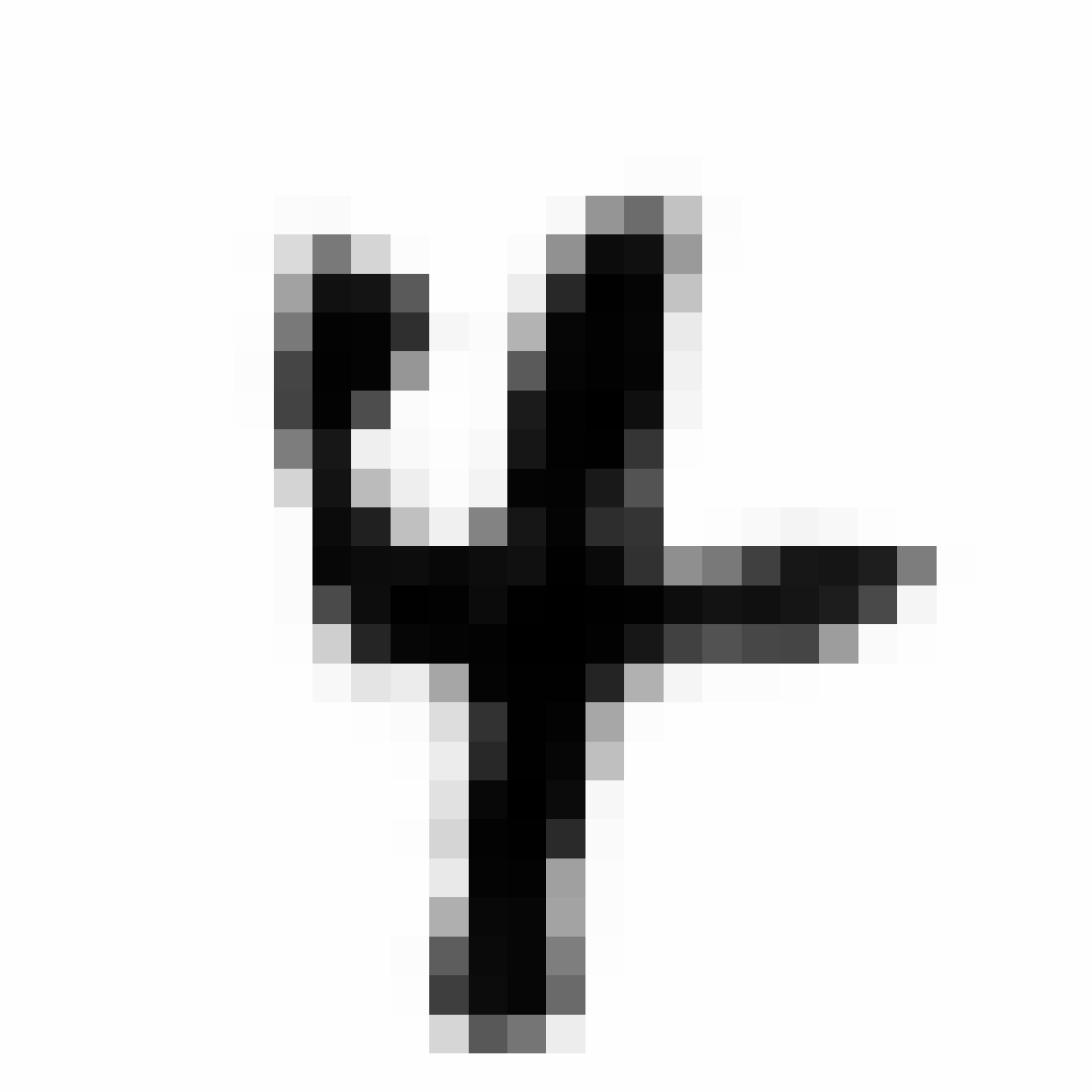
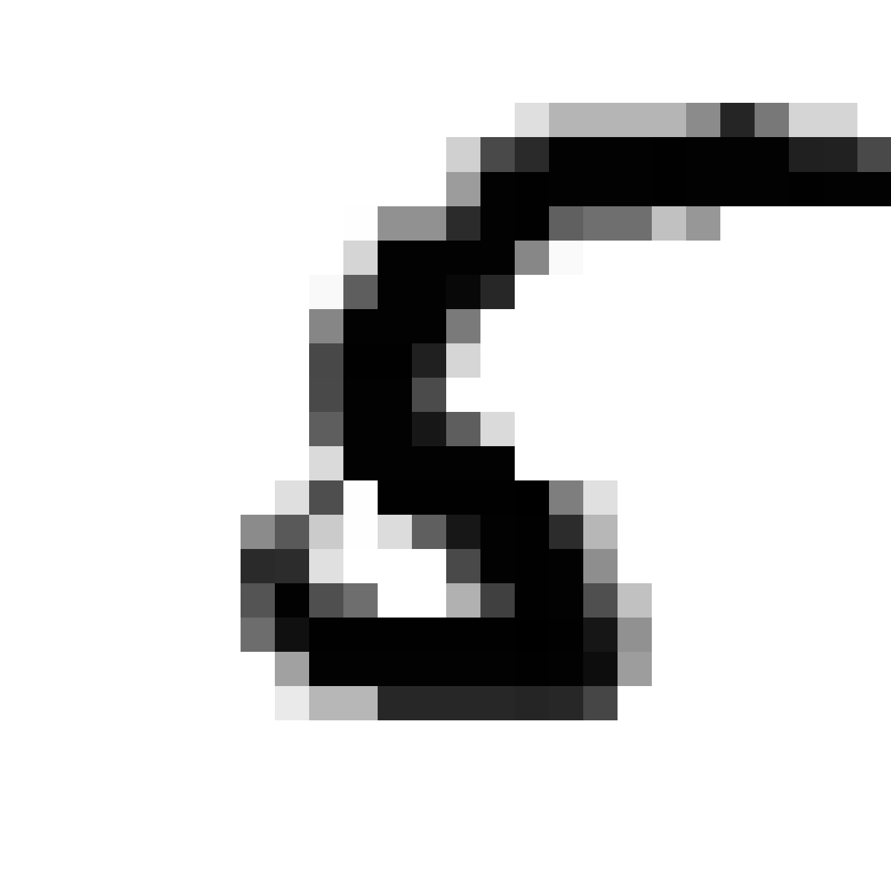
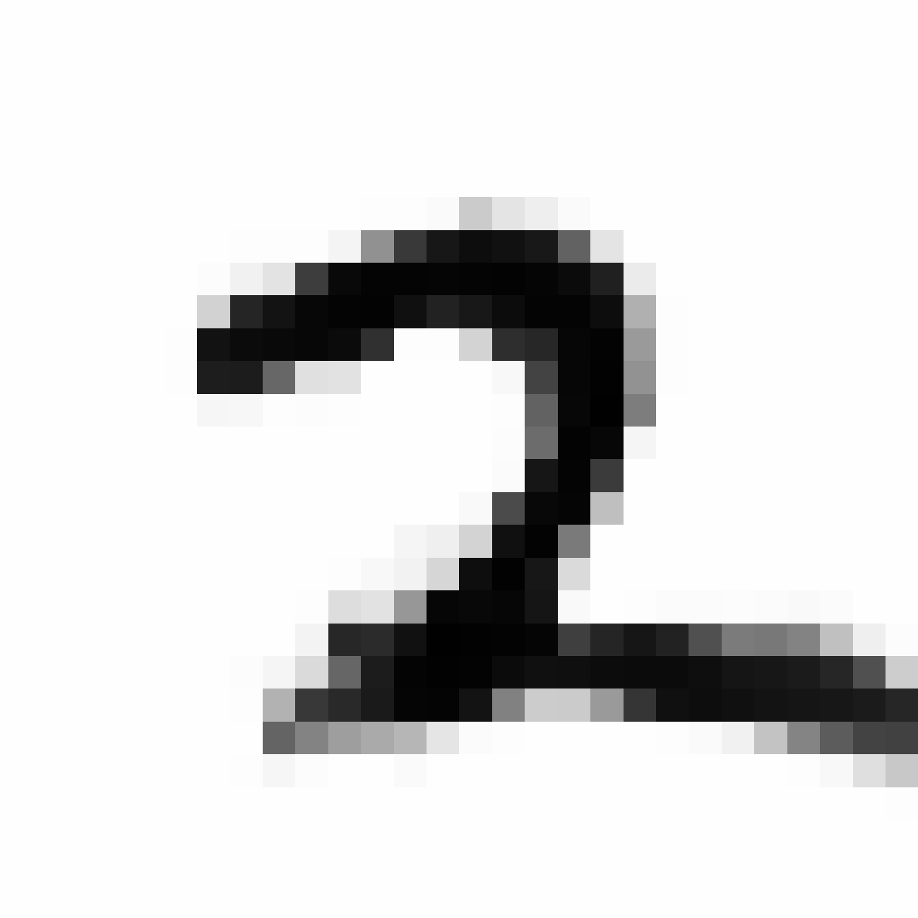
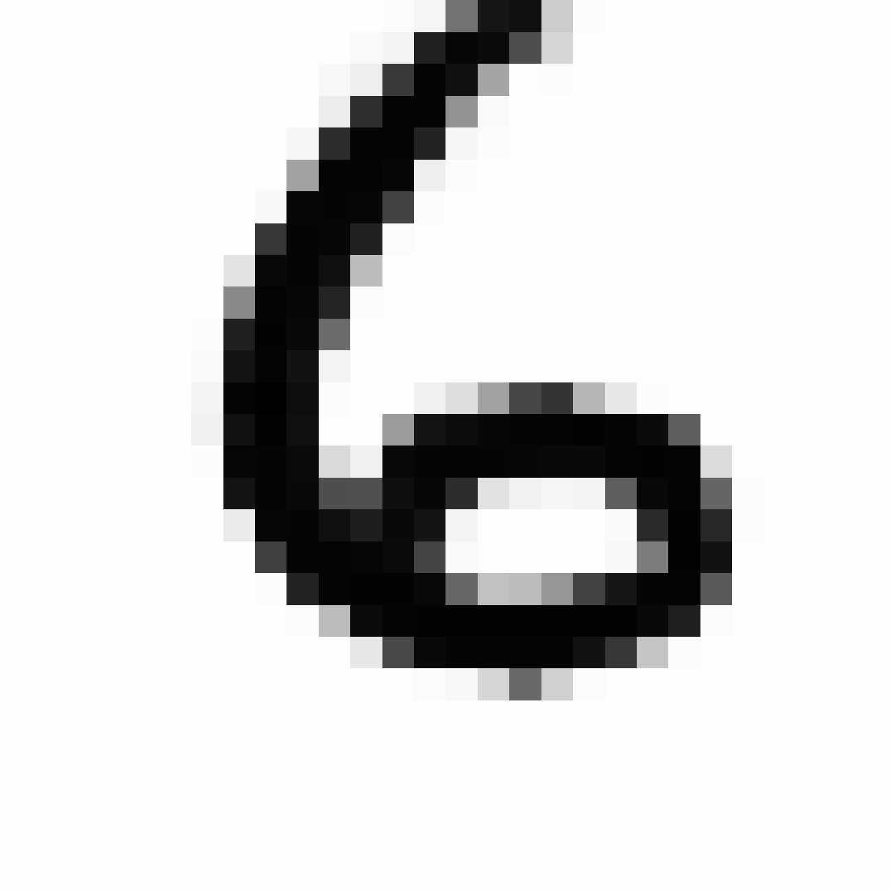
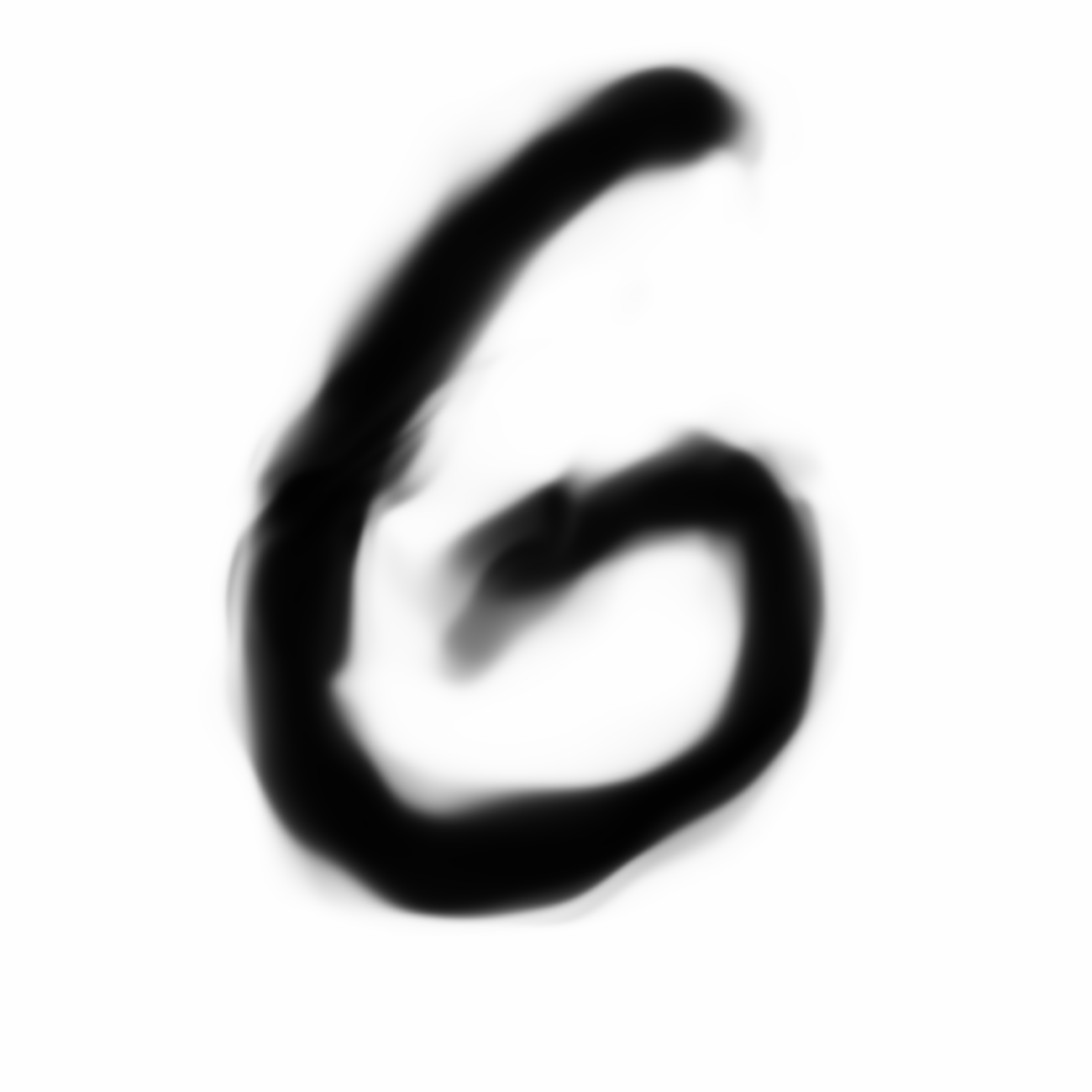
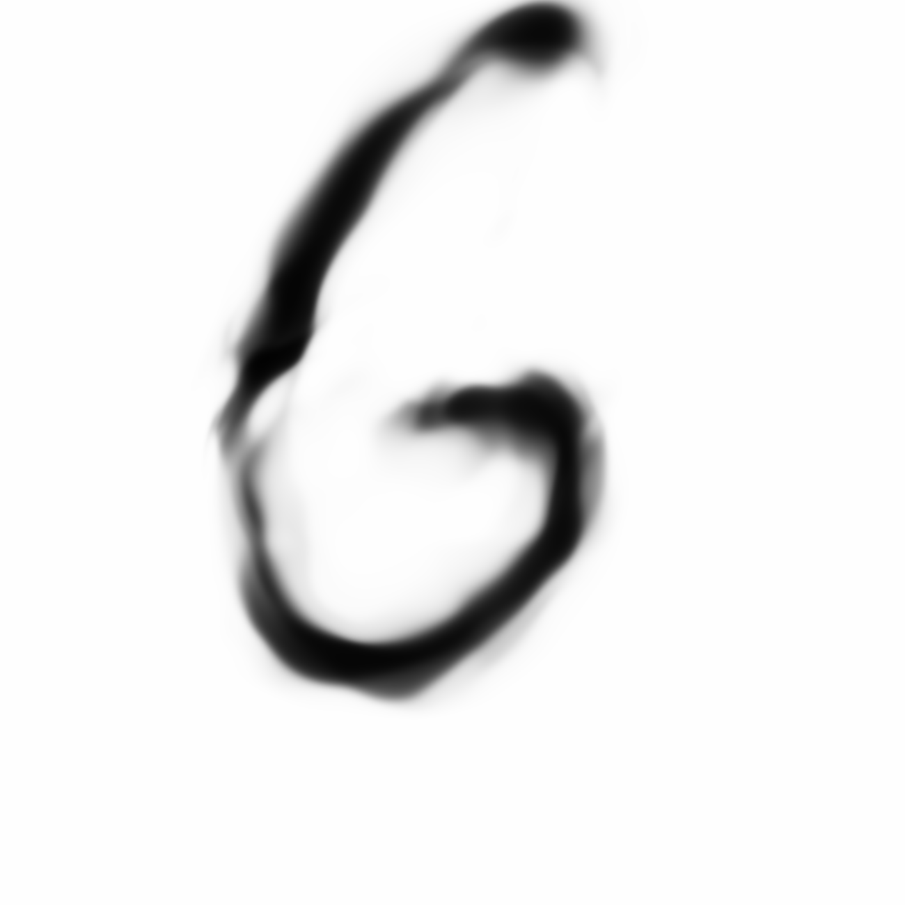
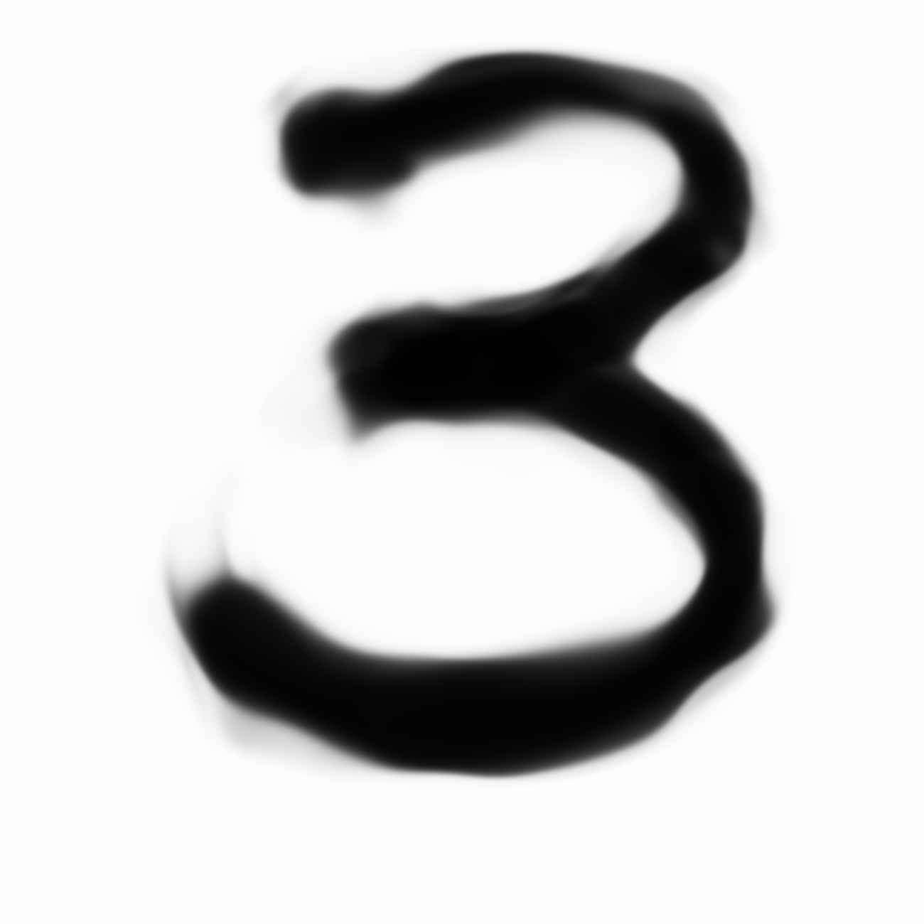
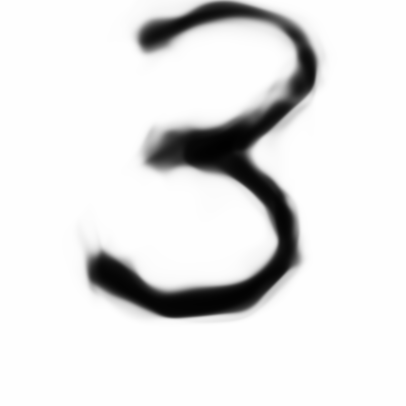
Below are more comparisons of autoencoded examples versus the originals. Sometimes the network makes mistakes, so it is not perfect. There is an example of a zero being misinterpreted as a six, and a three getting totally messed up. You can try to generate your own writing samples and feed an image into IPython to see what autoencoded examples get generated. Maybe in the future I can make a javascript demo to do this.
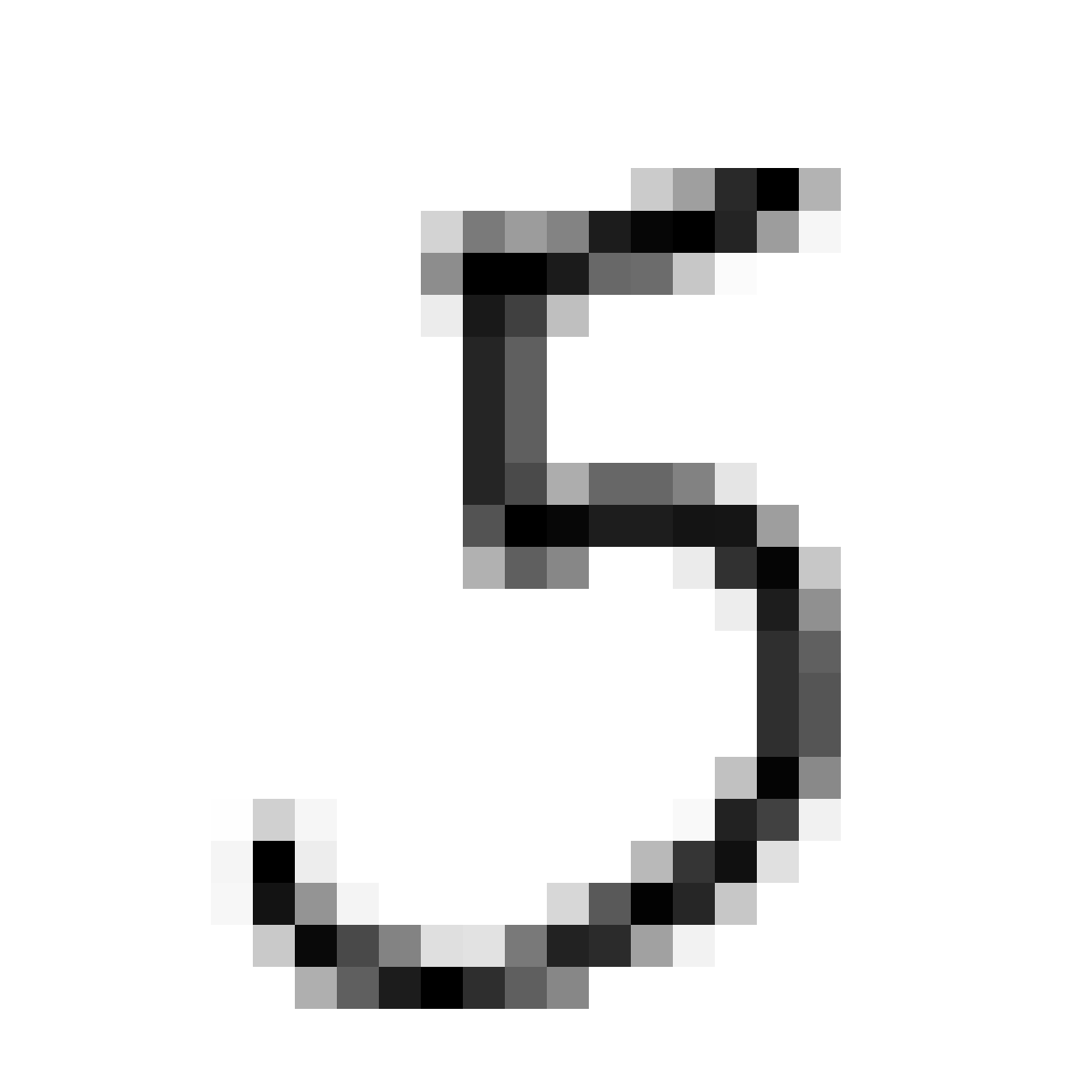
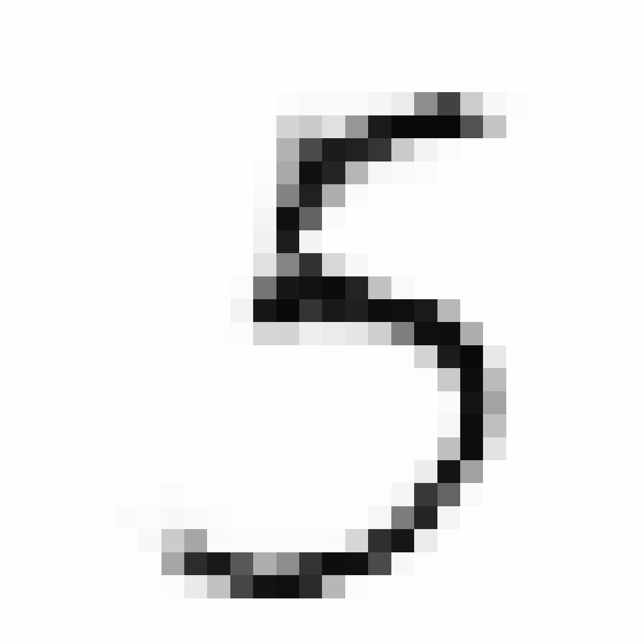
Autoencoded Samples
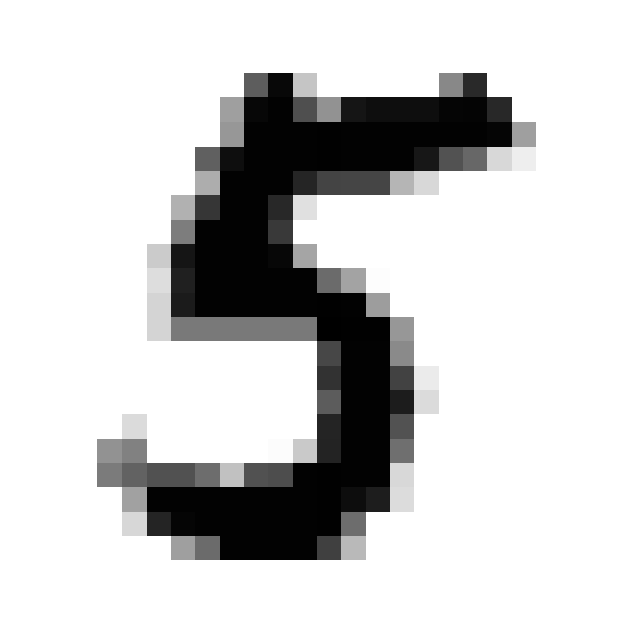
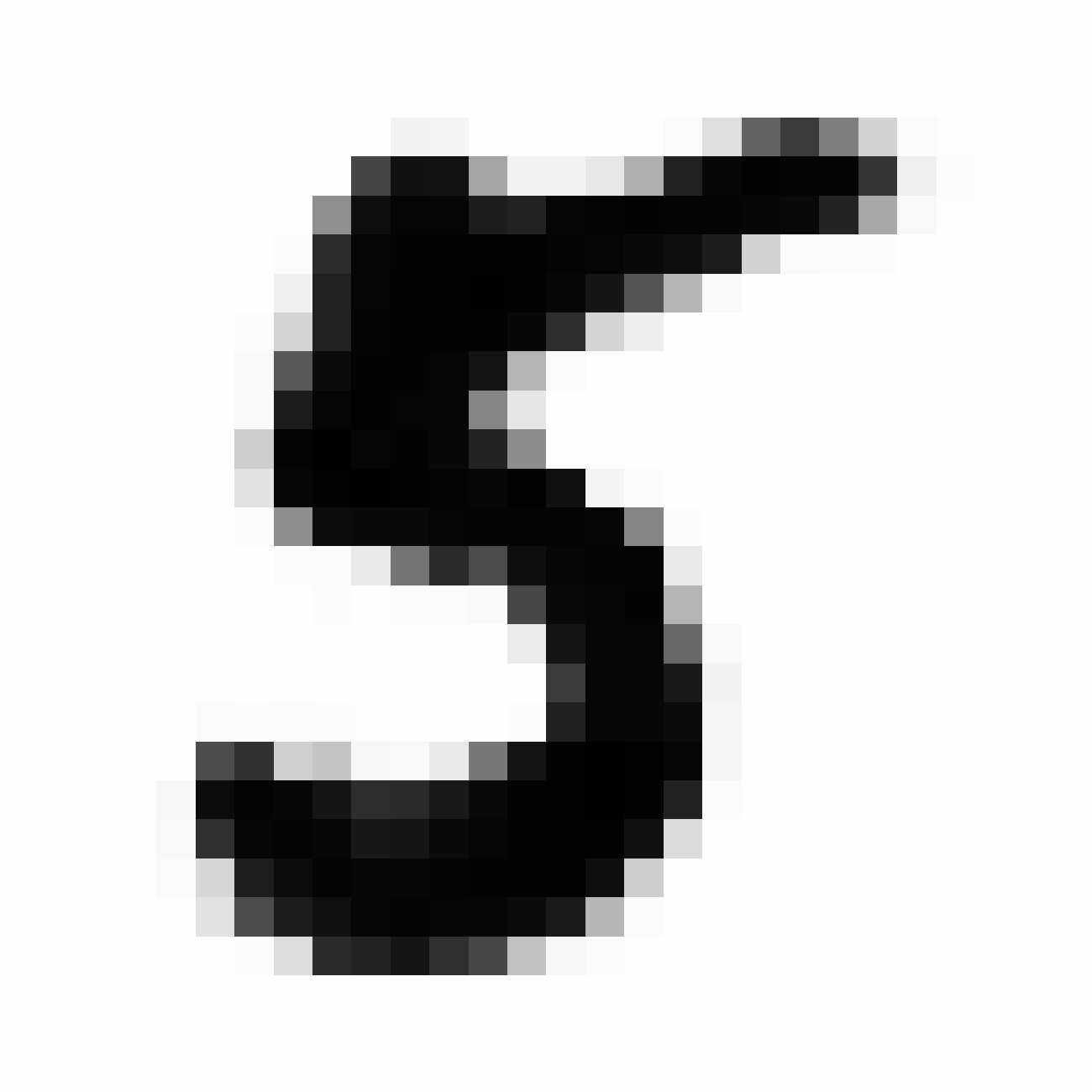
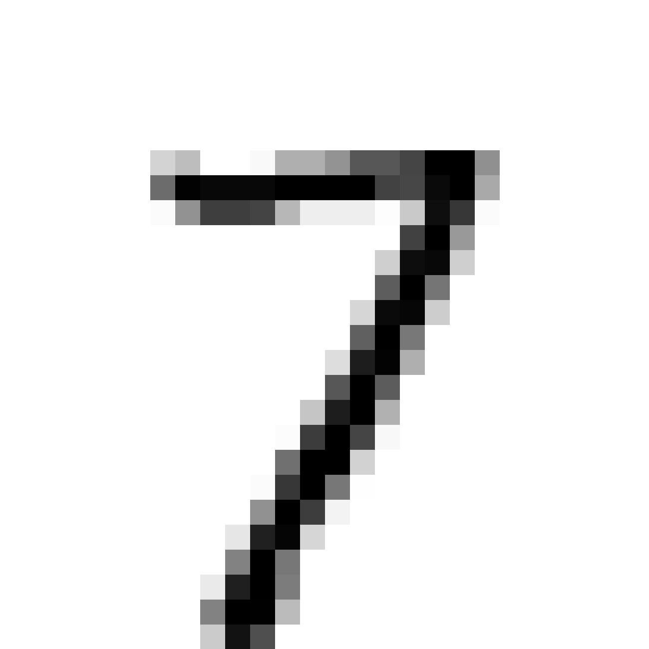
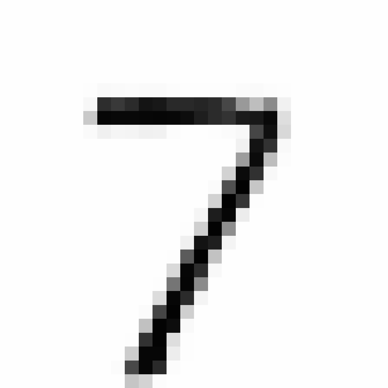
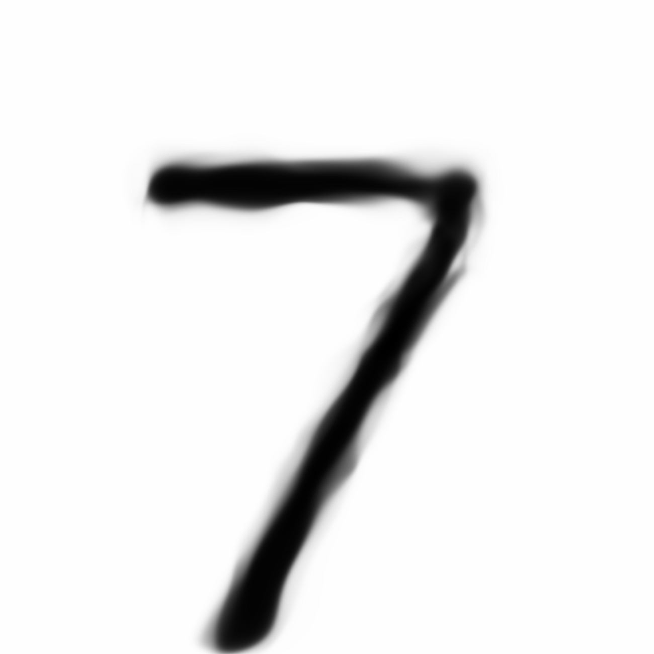
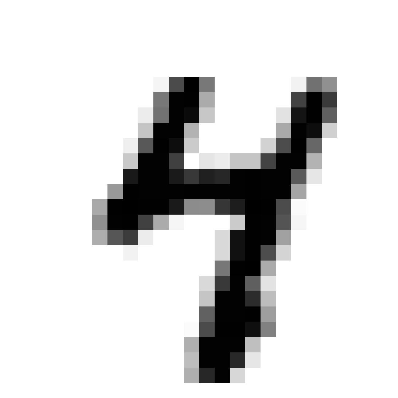
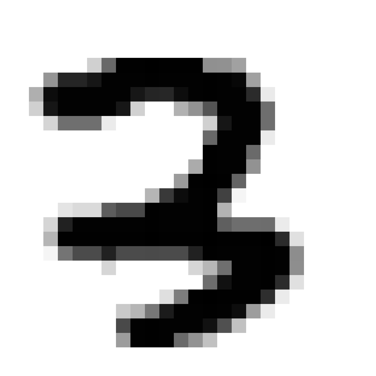
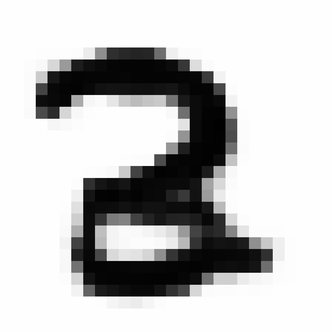
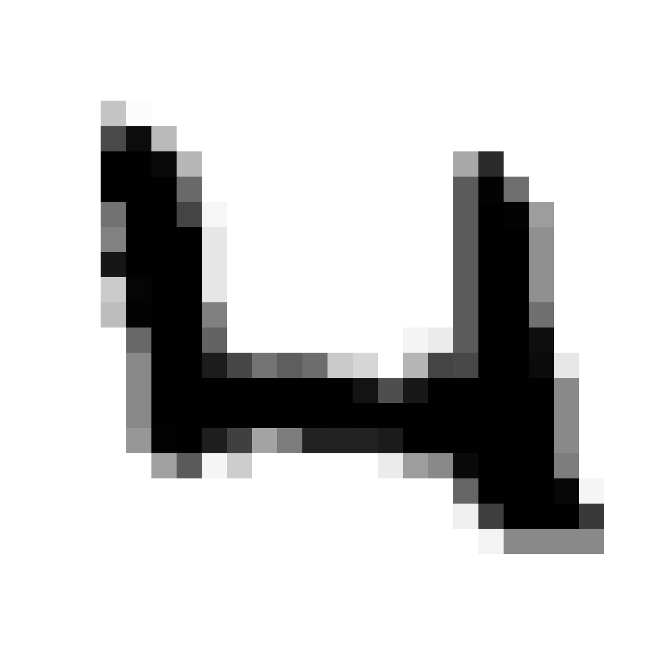
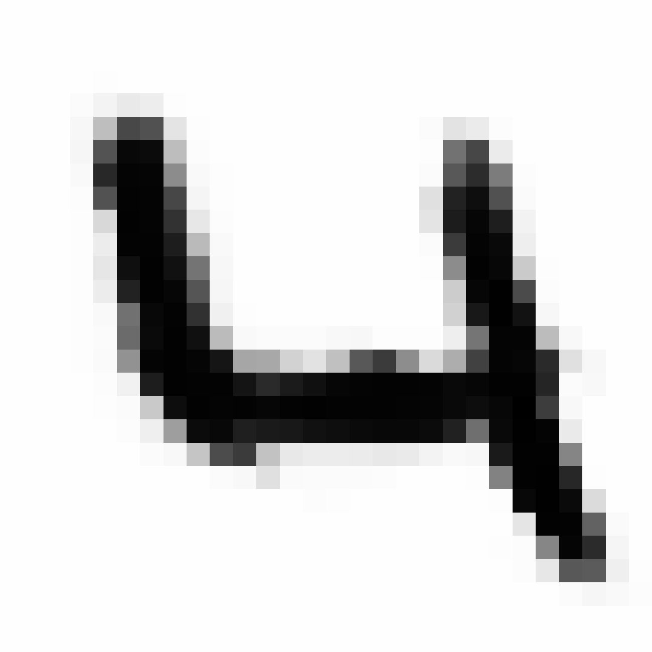
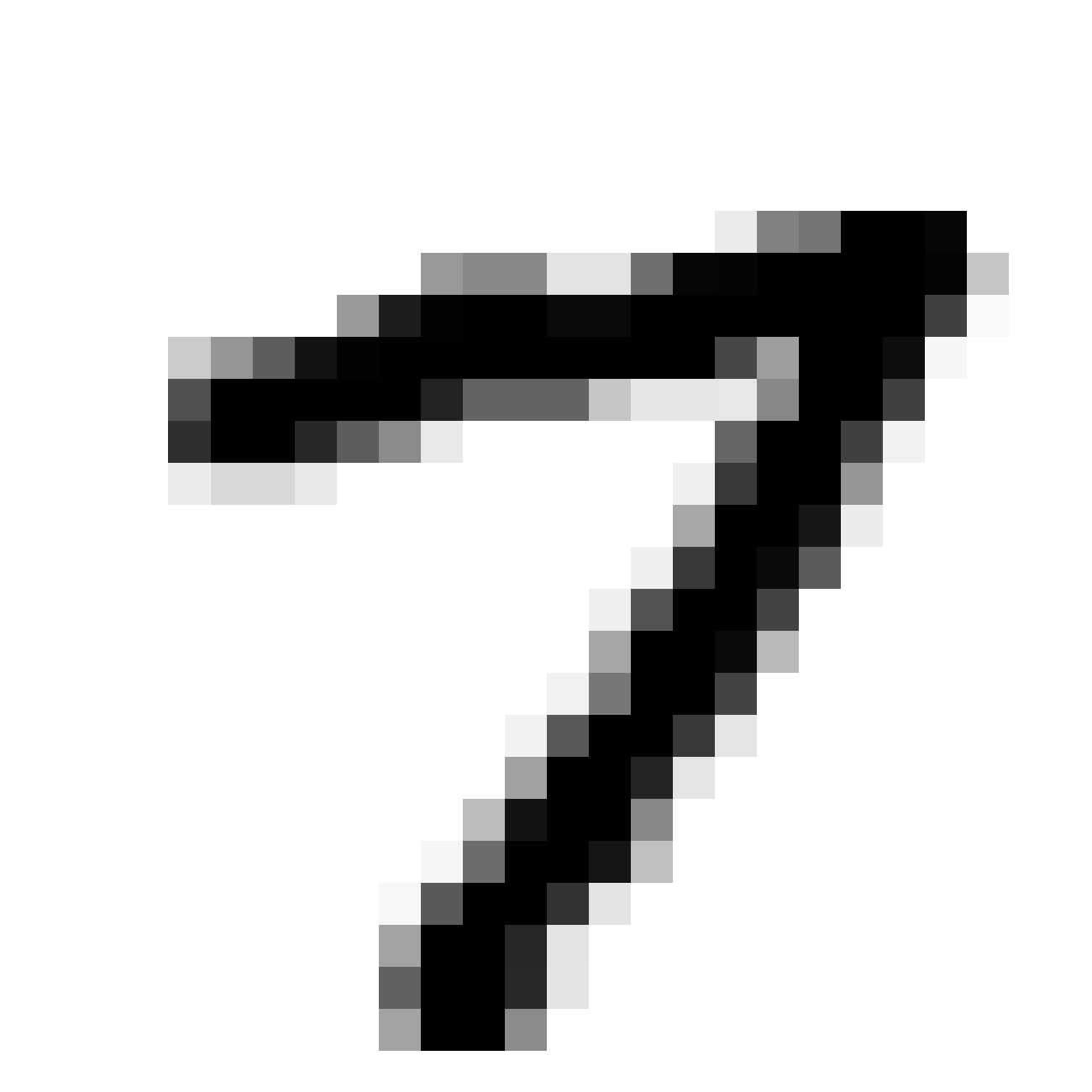
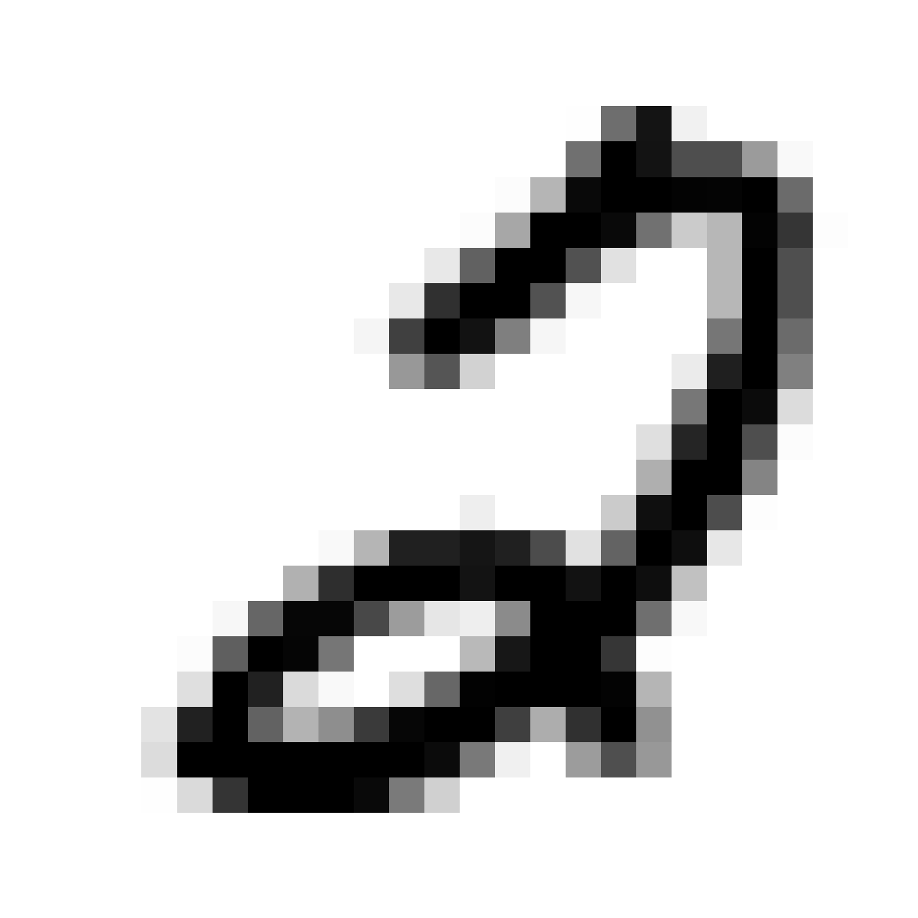
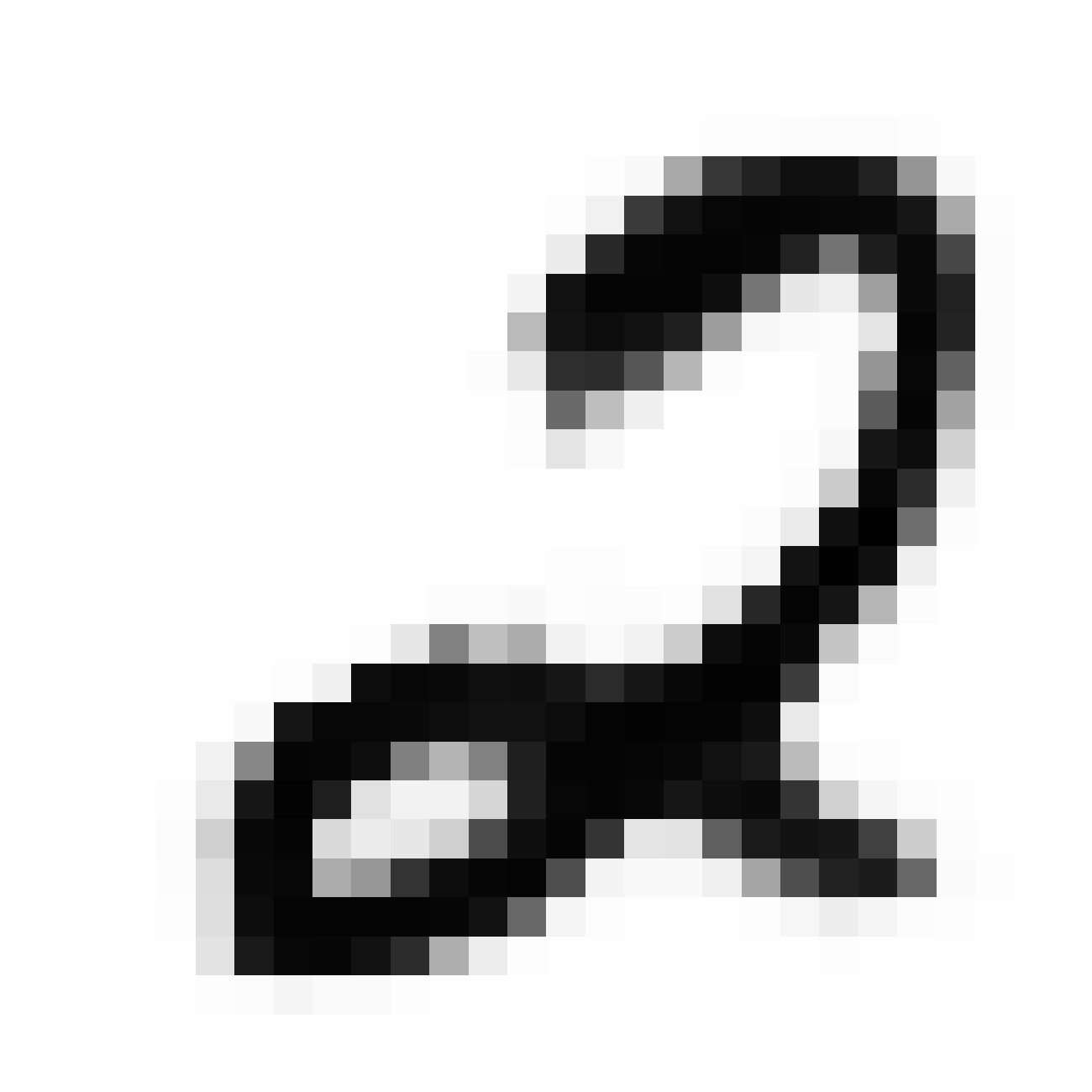
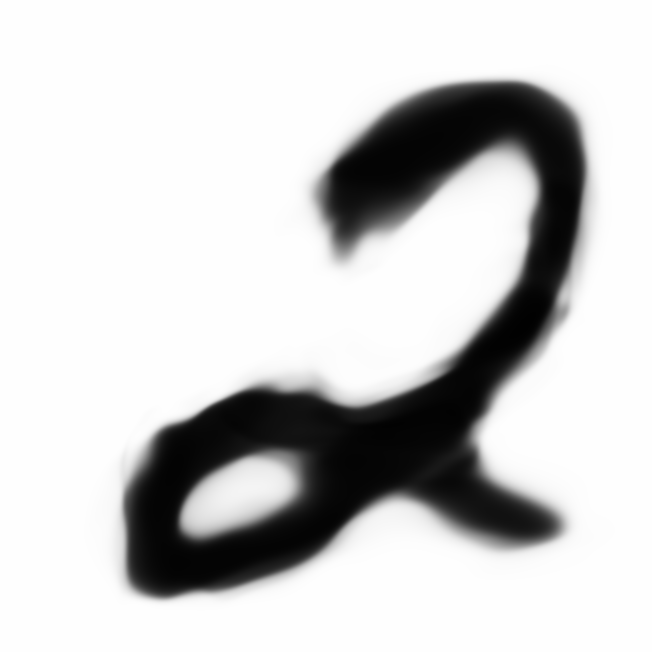
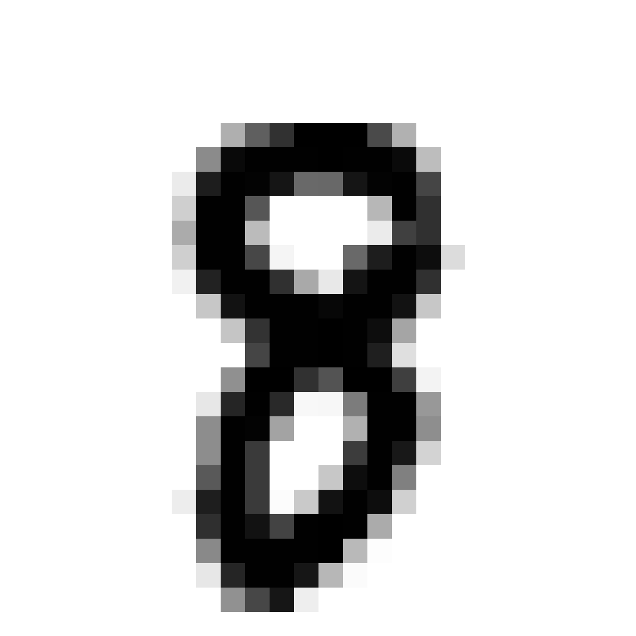
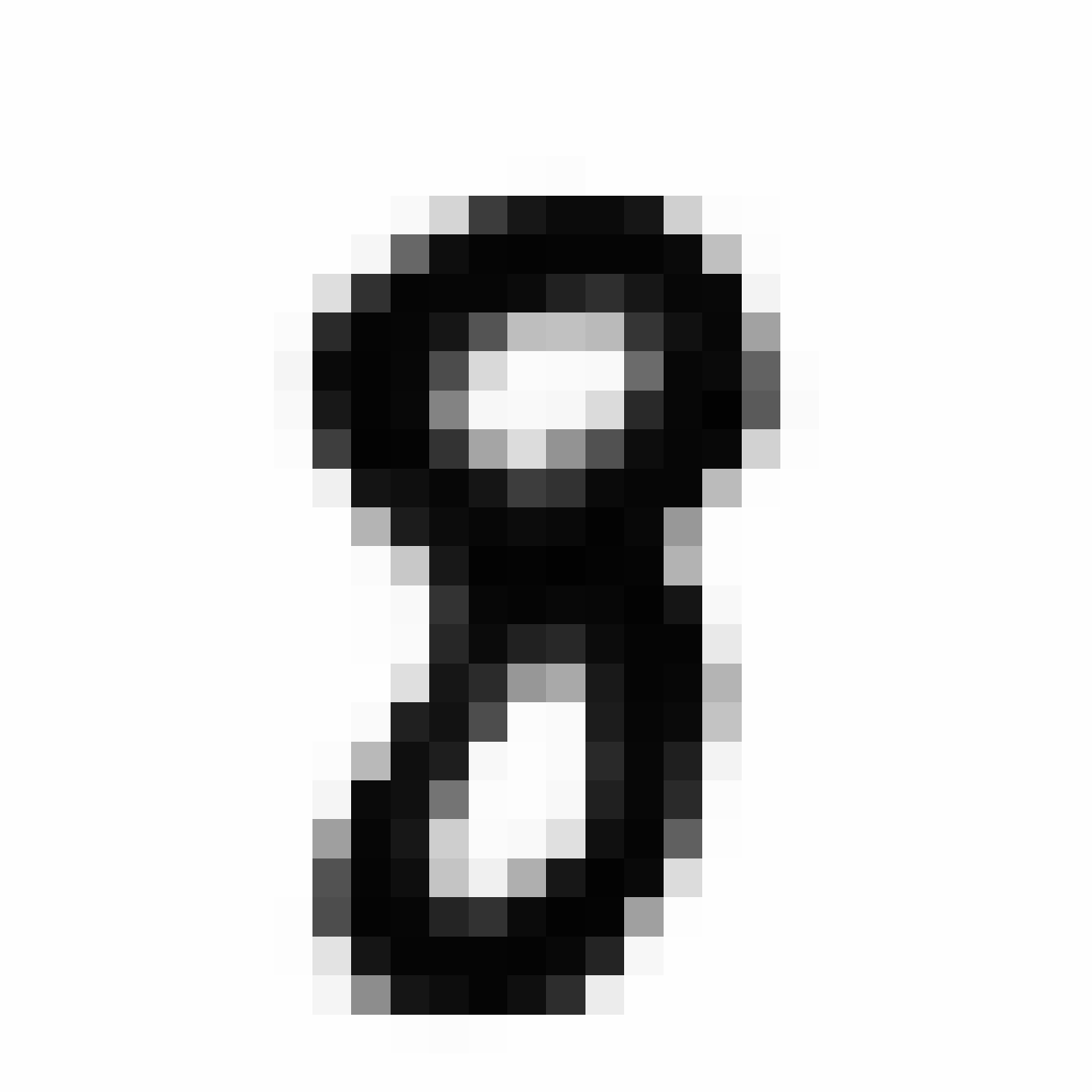
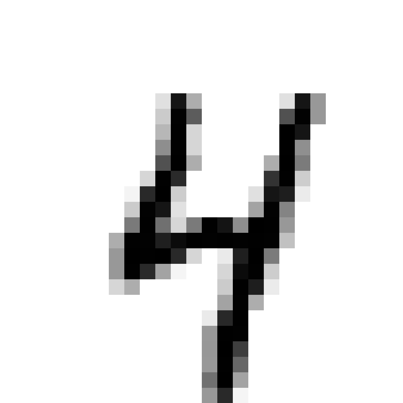
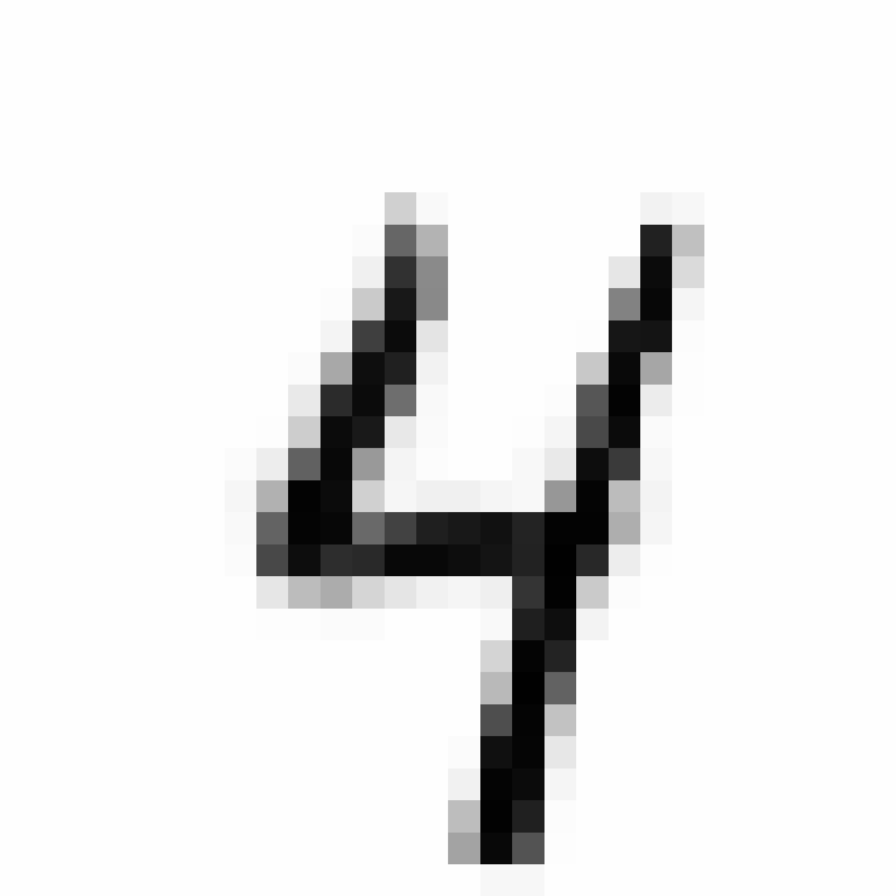
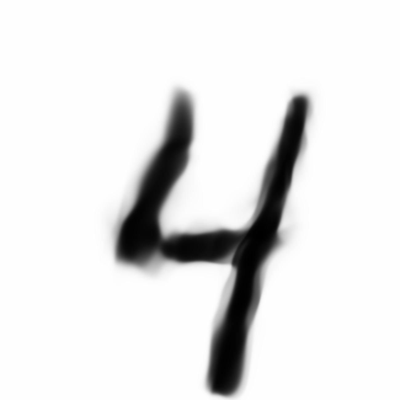
| MNIST Sample (26x26) | CPPN Output (26x26) | CPPN Output (1300x1300) |
|
|
|

|
|
|
|
|

|
|

|
|

|
|
|
|
|
|
|
|
|
|
|
|
|
|
|
|
|
|
|

|
|
|

|
|
|
|
|
|
|
|
|
|
|
|

|
|

|
|
|
|
|
|
|

|
|
|
|
|
|

|
|
|
|
|
|

|
|
|
|
|
|
|
|

|
|
|

|
|
|
|
|
|
|
|
|
As discussed earlier, the Latent Z Vector can be interpreted as a compressed coded version of actual images, like a non-linear version of PCA. Embedded in these 32 numbers is information containing not only the digit the image represents, but also other information, such as size, style and orientation of the image. Not everyone writes the same way, some people write it with a loop, or without a loop, and some people write digits larger than others, with a more aggressive pen stroke. We see that the autoencoder can capture most of these information successfully, and reproduce a version of the original image. An analogy would be a person looking at an image, and taking down notes to describe an image in great detail, and then having another person reproduce the original image from the notes.
Latent Vector Arithmetic
An interesting property that has been discovered from previous papers is that we can perform arithmetic on the Z-vectors to generate new images with interesting properties derived from the arithmetic. For example, if you encode the image of two women, where one lady is smiling and another lady looks pissed off, and take the difference between these two latent vectors and add this difference to the latent vector of an encoded image of an angry guy, you can generate a picture of this guy in his happy state. This is a little surprising because the process of encoding and decoding is highly non-linear, but I guess within certain bounds a certain amount of linearity holds. This phenomenon has been tested with VAE, GAN, and DCGAN where the pixels are generated directly. Let’s see if we see this work in the CPPN version of GAN-VAE.
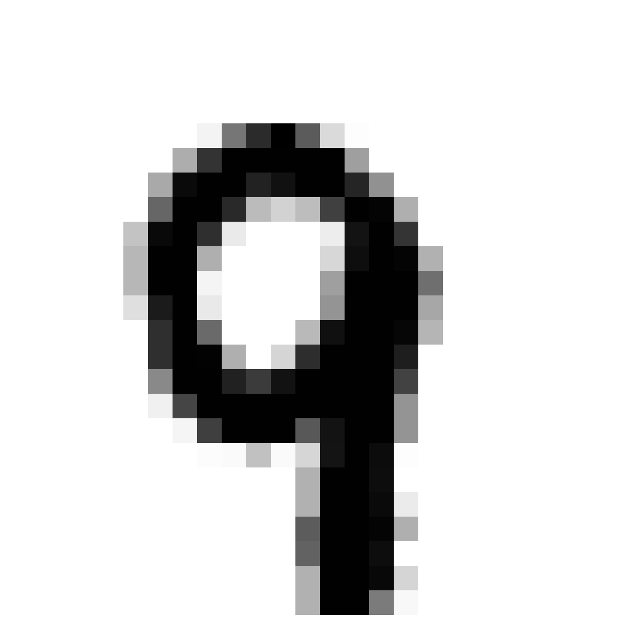
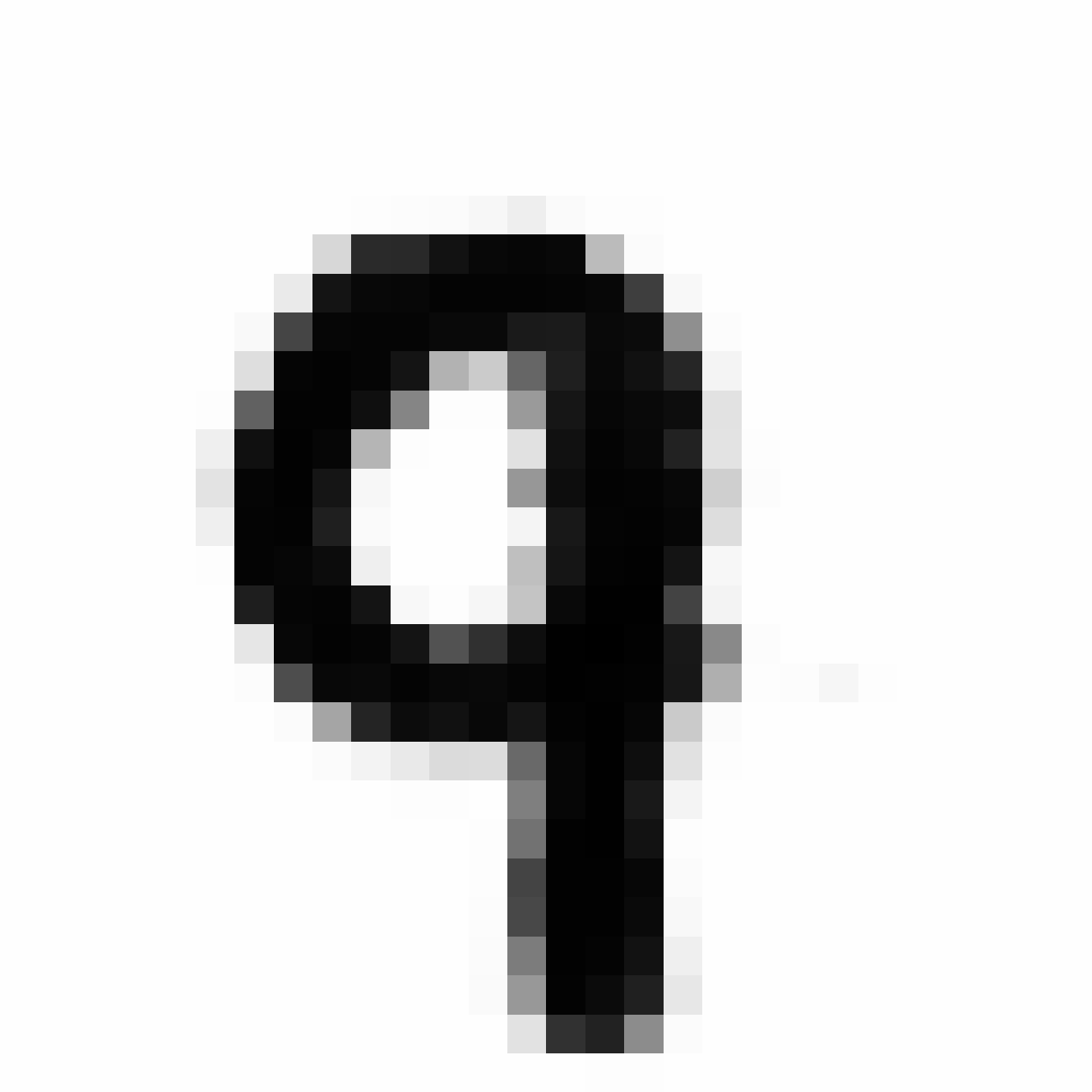
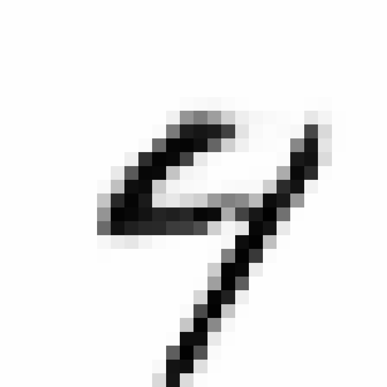
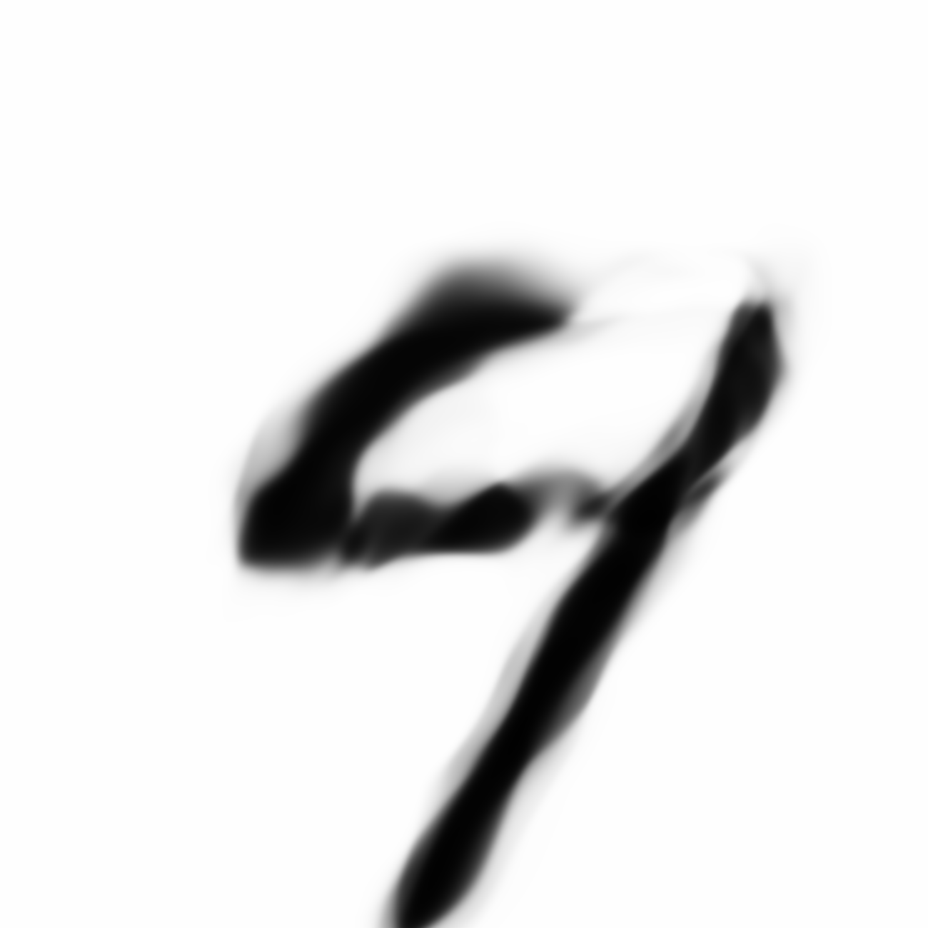
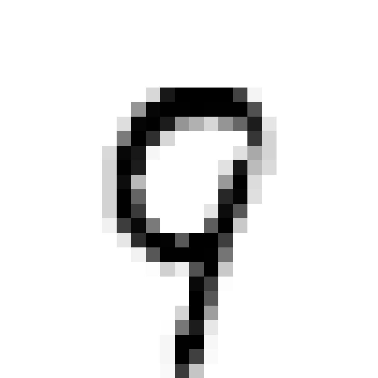
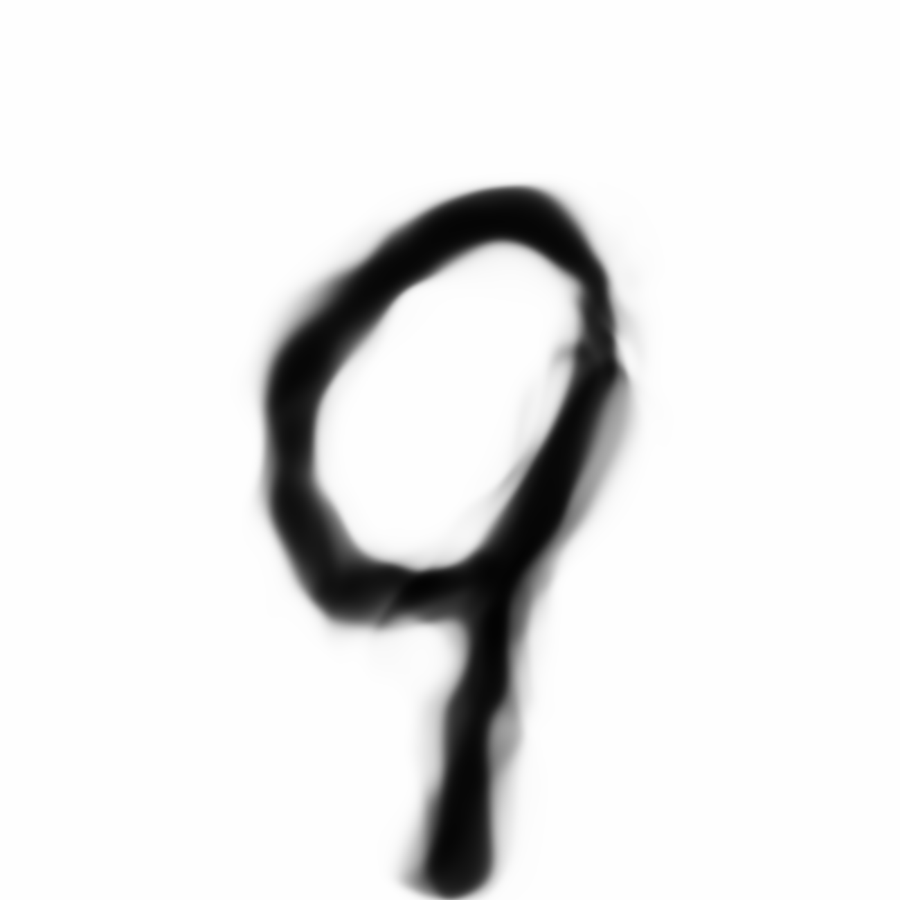
First, let’s get a random example of a from MNIST, and show the autoencoded version.
1
2
3
m = sampler.get_random_specific_mnist(9) # get a random picture of 9 from mnist dataset
z_9 = sampler.encode(m)
sampler.show_image_from_z(z_9)
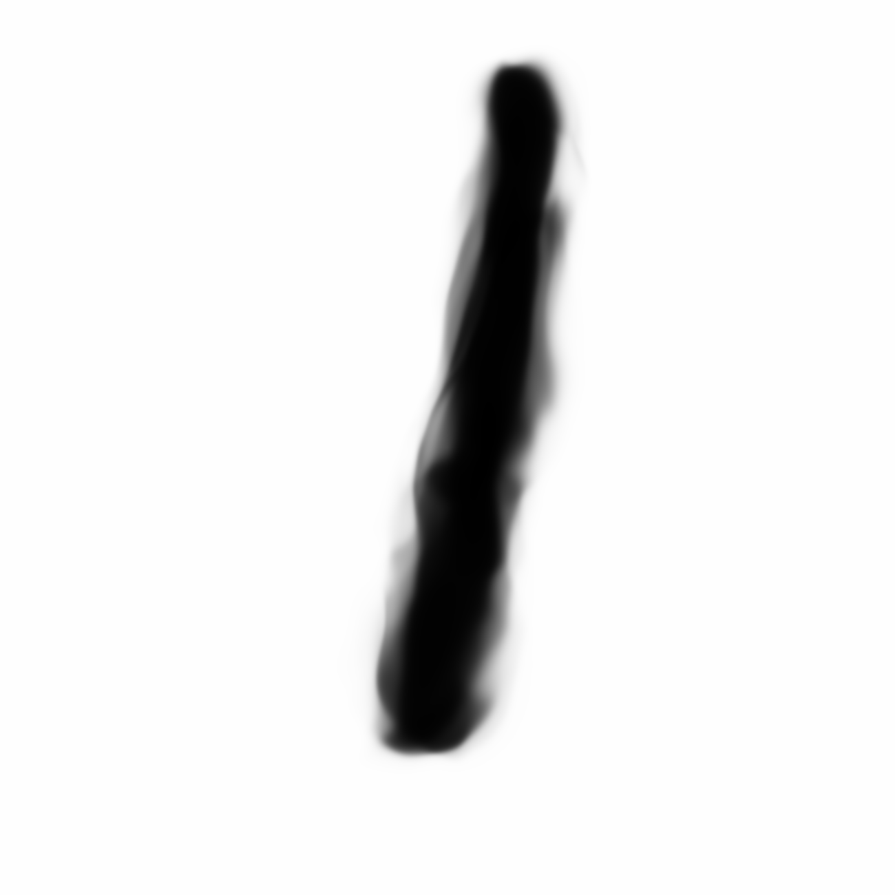
Then, let’s get two random examples of a from MNIST, and show the autoencoded versions.
1
2
3
4
z_1_before = sampler.encode(sampler.get_random_specific_mnist(1))
sampler.show_image_from_z(z_1_before)
z_1_after = sampler.encode(sampler.get_random_specific_mnist(1))
sampler.show_image_from_z(z_1_after)
z_1_before
|
z_1_after
|
|
|
We notice that one sample of is slanted compared to the other sample. We can take the difference of these two Z-vectors of , and add the result to the original Z-vector of and see what we get.
1
2
z_9_alter = z_9 + (z_1_after - z_1_before)
sampler.show_image_from_z(z_9_alter)
We see that the altered is also slanted in sort of the same way. We can try with other examples too.
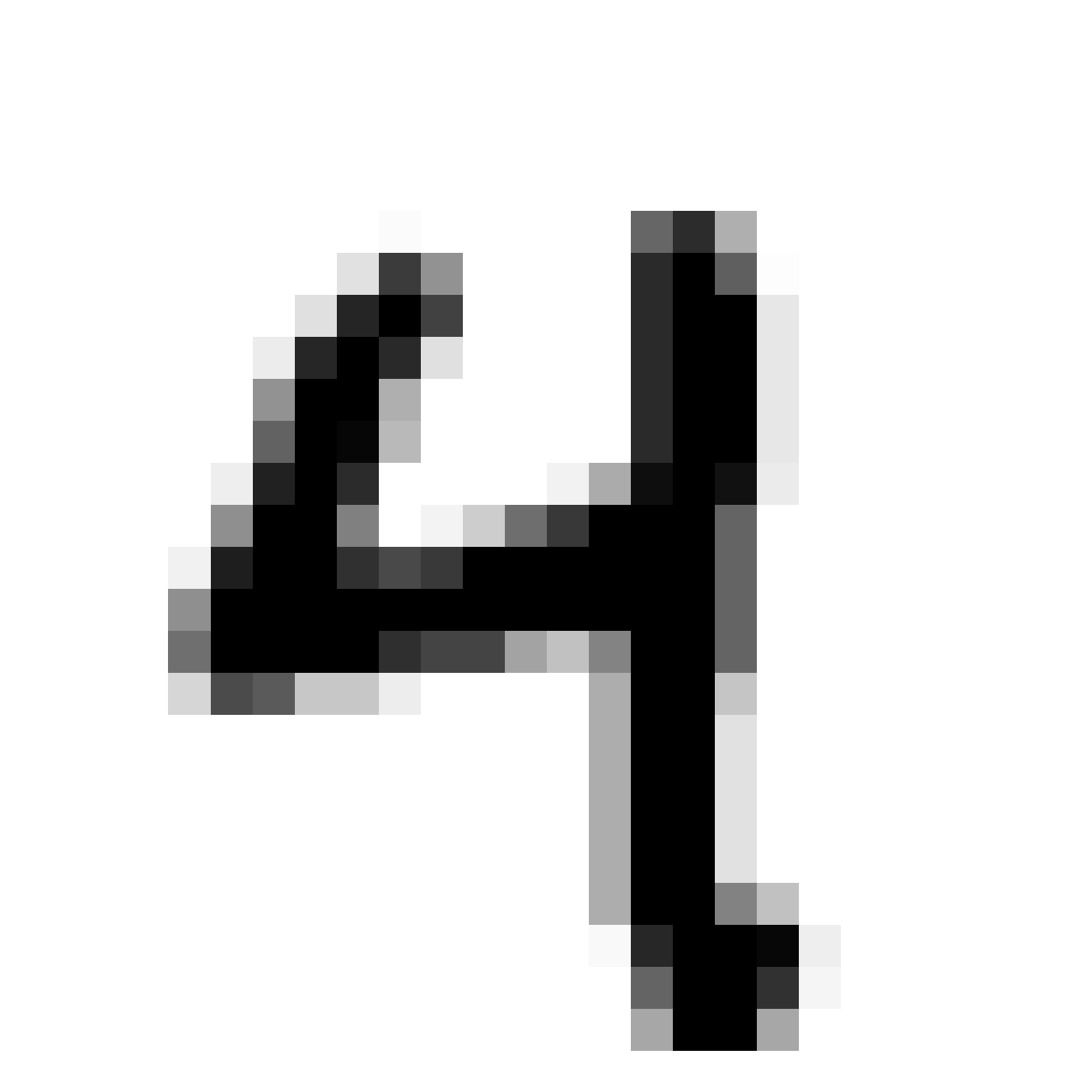
Below, we try to modify a normal looking by adding in the difference of a wide and narrow .
1
2
z_2 = sampler.encode(sampler.get_random_specific_mnist(2))
sampler.show_image_from_z(z_2)
1
2
3
4
z_5_before = sampler.encode(sampler.get_random_specific_mnist(5))
sampler.show_image_from_z(z_5_before)
z_5_after = sampler.encode(sampler.get_random_specific_mnist(5))
sampler.show_image_from_z(z_5_after)
z_5_before
|
z_5_after
|
|
|
1
2
z_2_alter = z_2 + (z_5_after - z_5_before)
sampler.show_image_from_z(z_2_alter)
For some reason, the narrower version of is written without the loop as the original version.
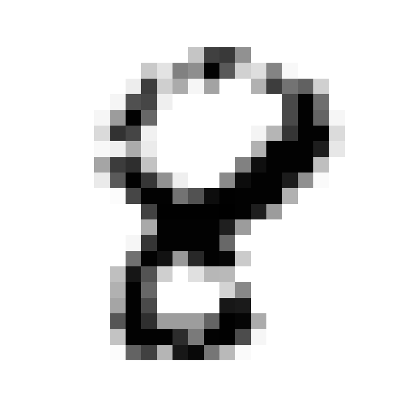
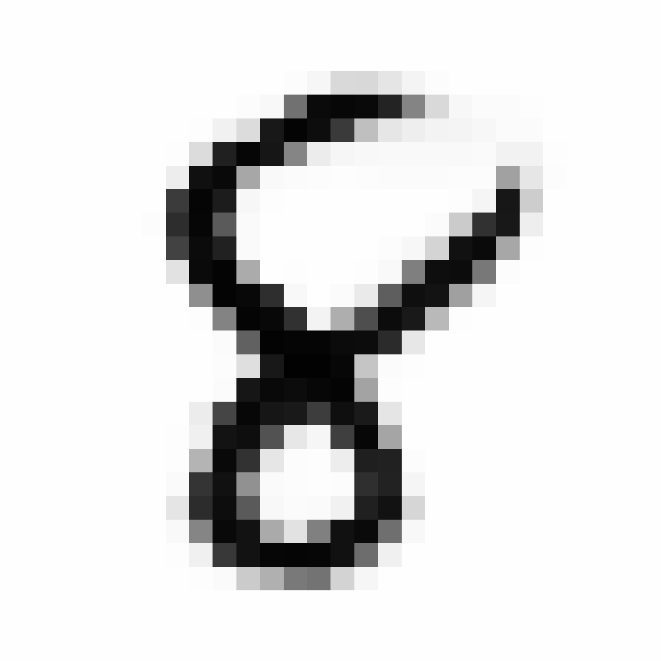
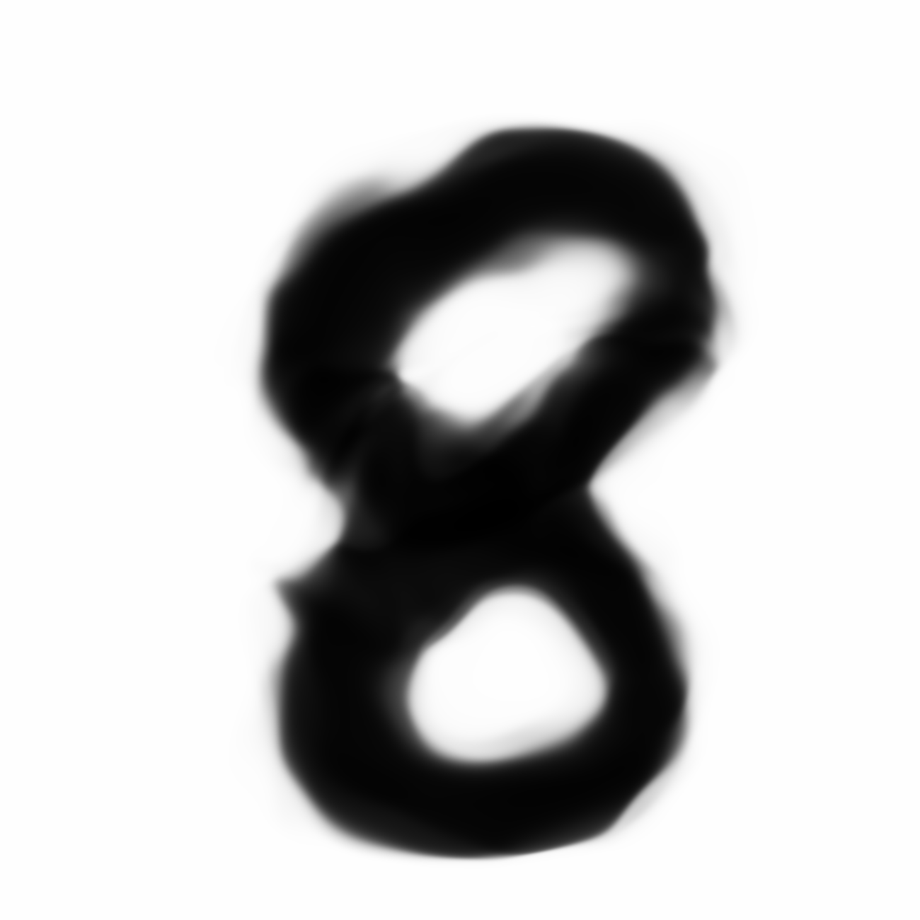
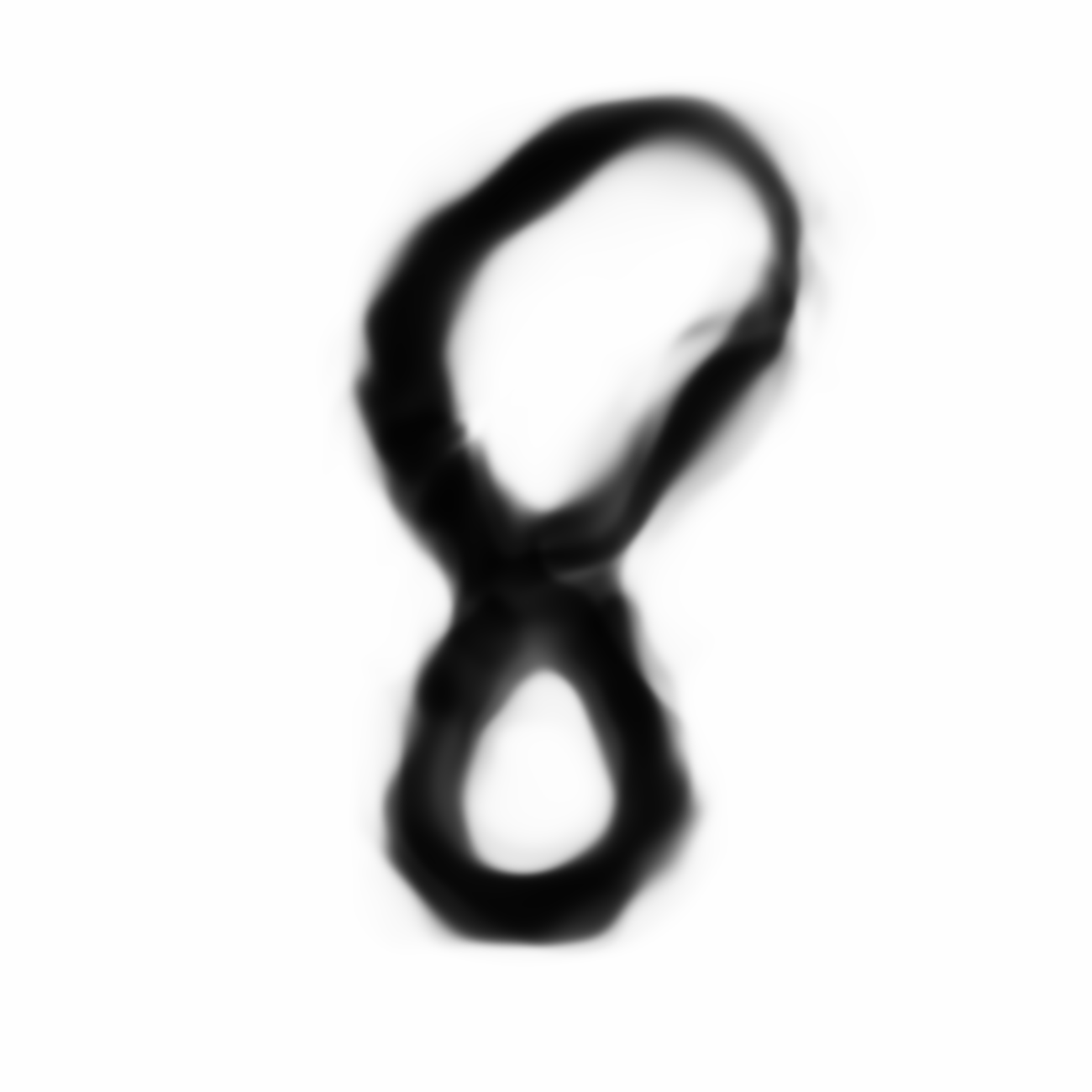
Some more examples involving style. We choose a fat and skinny , and use their latent-space difference to make a normal and fatter or skinnier.
z_fat_8
|
z_skinny_8
|
|
|
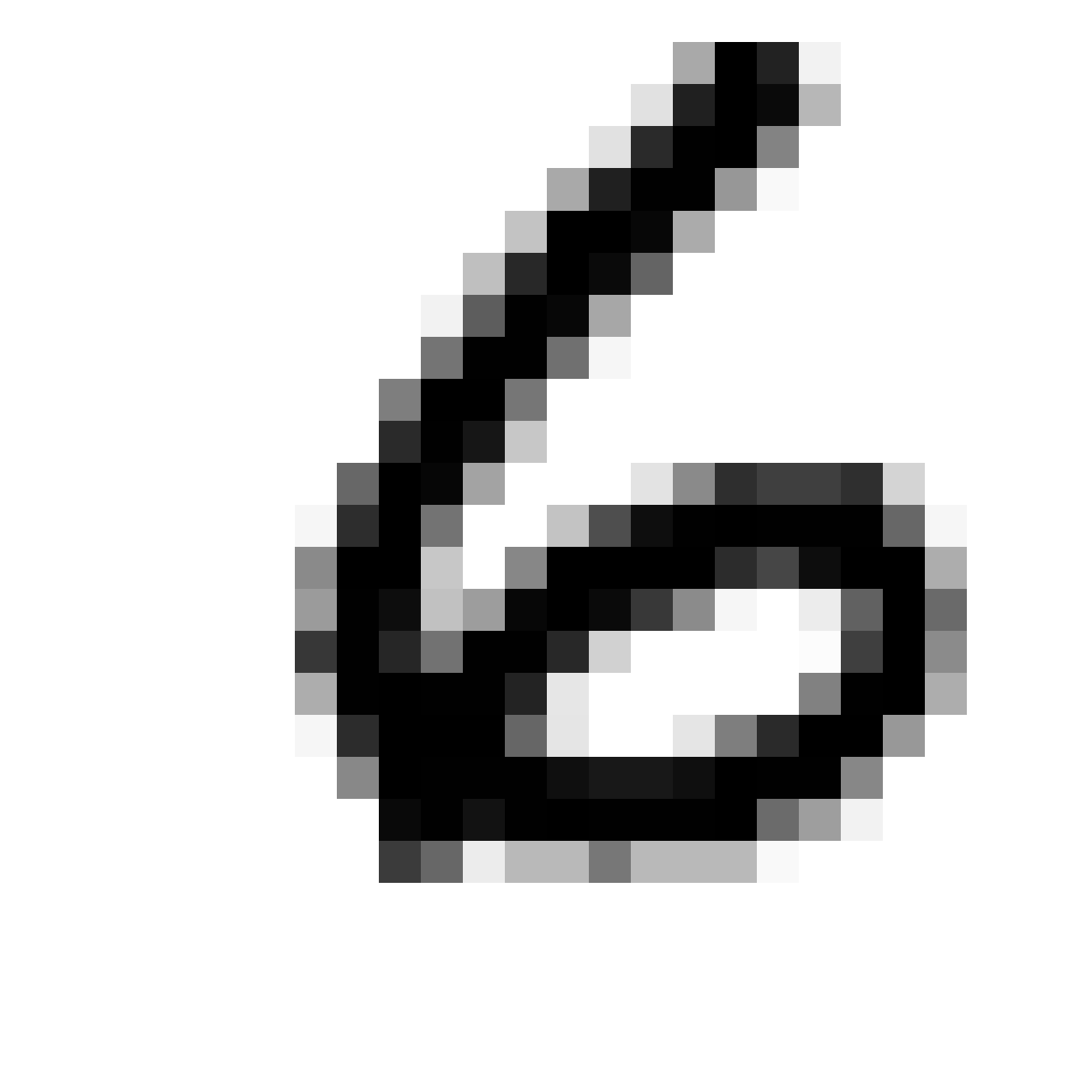
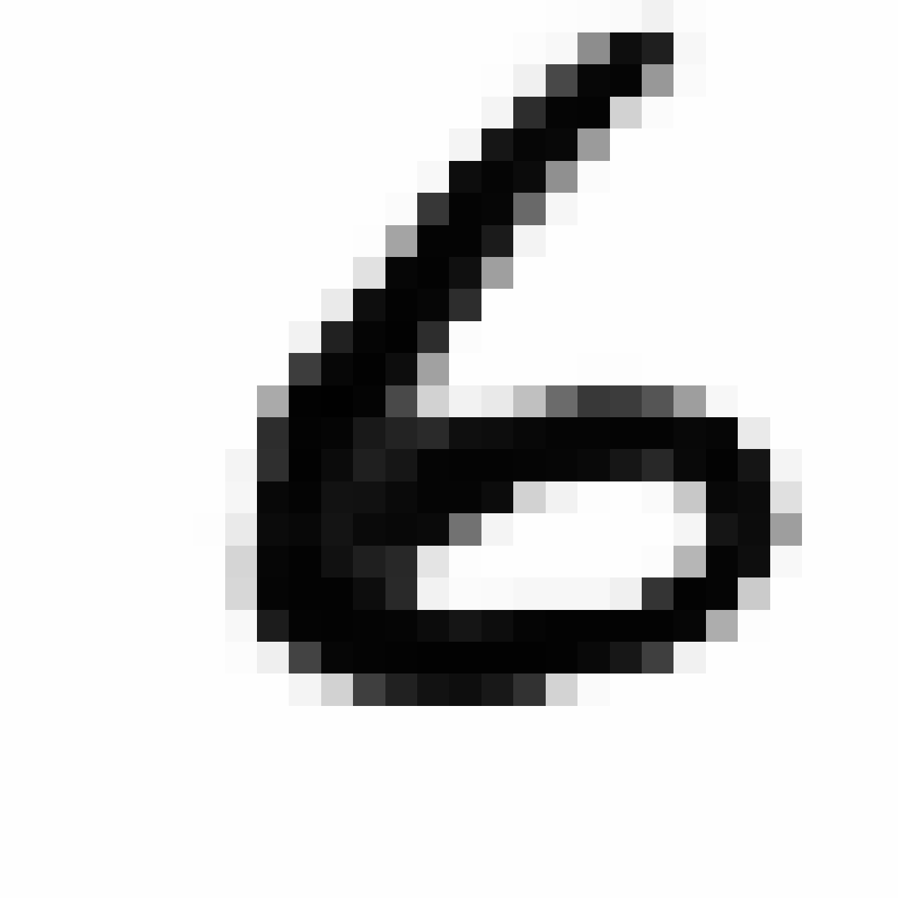
z_6
|
z_6+(z_skinny_8-z_fat_8)
|
|
|
z_3
|
z_3+(z_skinny_8-z_fat_8)
|
z_3+(z_fat_8-z_skinny_8)
|
|
|
|
Animations
I’ve also written some helper methods to visualise the transition from one latent state to another, and we can use these methods to create animated .gif files. For example, this is how to create an animation of a morphing to a , and then to a , and back to a , with a sinusoidal time effect:
1
2
3
4
5
6
7
8
z_2 = sampler.encode(sampler.get_random_specific_mnist(2))
z_9 = sampler.encode(sampler.get_random_specific_mnist(9))
z_0 = sampler.encode(sampler.get_random_specific_mnist(0))
x_array_2to9 = sampler.morph(z_2, z_9, sinusoid = True)
x_array_9to0 = sampler.morph(z_9, z_0, sinusoid = True)
x_array_0to2 = sampler.morph(z_0, z_2, sinusoid = True)
x_array = x_array_2to9 + x_array_9to0 + x_array_0to2
sampler.save_anim_gif(x_array, 'output_filename.gif', duration = 1.0 / 10.0)
Conclusions and Future Work
In the future I would like to attempt to train this algorithm on more interesting datasets compared to MNIST, which I think is a good first dataset to use.
We maybe able to train the network via curriculum learning as well, on higher resolution datasets. For example, first train the network to on a dataset scaled down to to 2x2 pixels. Once the training is satisficatory, we then train the same network on the same dataset at 4x4, then 8x8, and so on all the way to 1024x1024. The weights learned from the smaller set can be the initial set of weights used for the larger dataset, so on a very large network, the training path can be better directed from this type of curriculum training setup.
Some may argue that this CPPN is just doing nothing more than extrapolating between the pixels when the image is being expanded, and perhaps much simpler mathods can be used to accomplish this, but I think the concept of encapsulating the entire image generating process into a network that is able to generate an image with certain limitations (ie, it cannot directly dictate values for every pixel in the image), and being able to use gradient descent to train the encapsulted network to draw the concept of some object into an image is quite powerful.
For example, we can replace the CPPN, by another method, say a recurrent neural network that generates a set of vectorised points to represent an ink-brush image that can be converted to pixel format and compared to a training set. In other words, we can train a neural network to generate a set of instructions for a virtual paintbrush (which is limited in terms of the space of drawings it can create), to attempt to draw images that look like concepts in a dataset containing only images with pixels. This encapsulation framework allows us to train a network to think outside of pixel space first, and to be trained via back-propagation on examples from pixel space.
Finally, I want to figure out some alternatives to Maximum Likelihood as a training objective (it was used in the VAE part). I think a generated image that has a good score based on pixel vs pixel comparison to a training image does not necessarily imply that it looks natural to humans. This has been discussed before on Ferenc Huszár’s blog. The images trained on pure GAN looked punchier and has character, and I found them more interesting to look at compared to the smokey GAN+VAE combination, although the GAN+VAE combination looks much better than the pure VAE version which just looks like blurry images. I think further developments and improvements in adversarial training methodologies might allow us to get rid of Maximum Likelihood, and recent concepts such as Style and Structure GAN shows promise towards this direction.
Citation
If you find this work useful, please cite it as:
@article{ha2016generating,

  title   = "Generating Large Images from Latent Vectors",

  author  = "Ha, David",

  journal = "blog.otoro.net",

  year    = "2016",

  url     = "https://blog.otoro.net/2016/04/01/generating-large-images-from-latent-vectors/"

}