GitHub

This demo will attempt to use a genetic algorithm to produce efficient, but atypical neural network structures to classify datasets borrowed from TensorFlow Playground. Please try the demo here.

Motivation

A few weeks ago, Google released a Web Demo called TensorFlow Playground. If you haven’t played with it yet, I do encourage you to do so, as it is a really well designed web demo displaying the training progress of how a neural network handles a simple classification problem with a few dummy datasets. You get to customise many aspects of the network, such as the number of layers, neurons per layer and its activation function, initial input features, and so on.

One of the things that interested me was the feedback from users of that demo. People started experimenting with different neural network configurations, such as how many neural network layers are actually needed to fit a certain data set, or what initial features should be used for another data set. Which activation functions work better for which dataset?

In typical neural network-based classification problems, the data scientist would design and put together some pre-defined neural network, based on human heuristic, and the actual machine learning bit of the task would be to solve for the set of weights in the network, using some variants of stochastic gradient descent and the back propagation algorithm to calculate the weight gradients, in order to get the network to fit some training data under some regularisation constraints. The TensorFlow Playground demo captured the essence of this sort of task, but I’ve been thinking if machine learning can also be used effectively to design the actual neural network used for a given task as well. What if we can automate the process of discovering neural network architectures?

I decided to experiment with this idea by creating this demo. Rather than go with the conventional approach of organising many layers of neurons with uniform activation functions, we will try to abandon the idea of layers altogether, so each neuron can potentially connect to any other neuron in our network. Also, rather than sticking with neurons that use a uniform activation function, such as sigmoids or relu’s, we will allow many types of neurons with many types of activation functions, such as sigmoid, tanh, relu, sine, gaussian, abs, square, and even addition and multiplicative gates.

The genetic algorithm called NEAT will be used to evolve our neural nets from a very simple one at the beginning to more complex ones over many generations. The weights of the neural nets will be solved via back propagation. The awesome recurrent.js library made by karpathy, makes it possible to build computational graph representation of arbitrary neural networks with arbitrary activation functions. I implemented the NEAT algorithm to generate representations of neural nets that recurrent.js can process, so that the library can be used to forward pass through the neural nets that NEAT has discovered, and also to backprop the neural nets to optimise for their weights.

Introduction to Neuroevolution

Most students studying machine learning learn that in order to train a neural network, one should define an objective function to measure how well the neural network is performing some task, and to use back propagation to solve for the derivatives of this objective function with respective to each weight, and afterwards use these gradients to iteratively solve for a good set of weights for the neural network. This framework is known as end-to-end training.

While the back propagation algorithm is currently the most powerful method for many applications, it is certainly not the only method. There are other methods for coming up with neural network weights. For example, going to one extreme, one method is just to randomly guess the weights of a neural network until we get a set of weights that can help us perform some task.

Genetic algorithms is a very simple step beyond random guessing. It works as follows: Imagine if we have 100 sets of random weights for a neural network, and evaluate the neural network with each set of weights to see how well it performs a certain task. After doing this, we keep only the best 20 set of weights. We reshape each set of weights into one-dimensional arrays. Then, we can populate the remaining 80 set of weights by randomly choosing from the 20 that we kept, and applying a simple crossover and mutation operation to form a new set of weights:

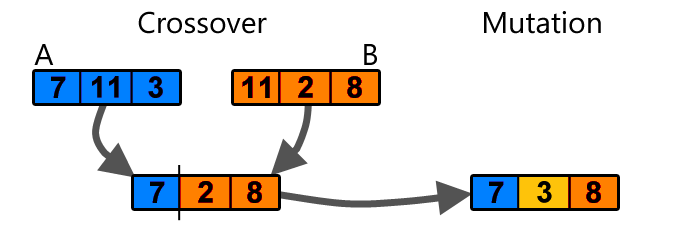
Simple example of crossover and mutation (image source)

The set of the new 80 weights will be some mutated combination of the top 20, and once we have a full set of 100 weights again, we can repeat the task of evaluating the neural network with each set of weights again and repeat the evolution process until we obtain a set of weights that satisfy our needs.

This type of algorithm is an example of Neuroevolution, and is very useful for solving for neural network weights when it is difficult to define a mathematically well behaved objective function, such as functions with no clear derivatives. Using this simple type of method in the past, I have managed to train neural networks to balance inverted pendulums, play slime volleyball, and get agents to collectively learn to avoid obstacles.

Although this method is easy to implement and easy to use, it doesn’t really scale well, especially when the size of the network is beyond a thousand connections. The volleyball agent’s brain only consists of a dozen or so activation functions. Modern methods such as Deep Q Learning, and policy gradients will also allow us to train a (much larger) network for these control tasks, or game playing tasks using back propagation. That being said, I bet my simple volleyball agent will still kick DQN’s ass :-)

Research in Deep Learning in the past few years have given us many useful tools to efficiently use backprop for many machine learning tasks. In addition to weight regularisation, we have dropout, rmsprop, batch normalisation, etc to name a few. So I feel that backprop will continue to be very useful part of training neural networks in the future, as researchers discover methods to frame many more problems into the end-to-end framework.

In addition to weight-search, Deep Learning research has also produced many powerful neural network architectures that are important building blocks. Historically, most neural network architectures had been hand-engineered by brilliant minds. For example, LSTM gates were hand-crafted to avoid the vanishing gradient problem for RNNs. Convnets were created to minimise the number of connections required for computer vision problems. ResNets were designed to be able to stack up many layers of neural nets effectively. Usually, after such novel architectures are discovered and adapted in mainstream academic research, other researchers would look back and realise how simple the discovery actually was and regret that they couldn’t be the first to come up with the idea.

I think neural network architecture design is an area where Neuroevolution can be a useful tool. Genetic algorithms do not stop at merely being able to discover neural network connection weights. It can also be extended to discover entire neural networks. I think getting computers to be able to automatically discover novel neural network architectures is a really cool idea, and so I created this simple demo to explore this concept.

Evolving Neural Network Topology

Neuroevolution of Augmenting Topologies (NEAT) is a method that can evolve new types of neural networks based on genetic algorithms. It was published more than a decade ago by Ken Stanley, and is popular amongst the small fringe community of AI researchers focused on evolutionary computing. Evolutionary computing is certainly not popular in mainstream machine learning research, where deep learning dominates. Deep learning researchers are like the pop idols in the AI community, while evolutionary computing researchers are more like some obscure garage indie metal bands that no one has heard of.

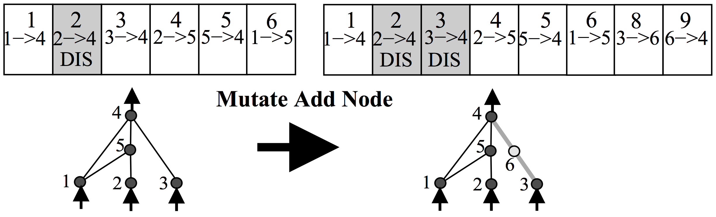
Anyways, the way NEAT works is to represent a neural network as a list of connections. At the beginning, the initial population of networks will have a very simple architecture, such as having each input signal and bias simply connect directly to the outputs with no hidden layers. In the mutation operation, there is some probability that a new neuron will get created. A new neuron will be placed in between an existing connection, hence a new connection will be created after the introduction of a new neuron, like the below:

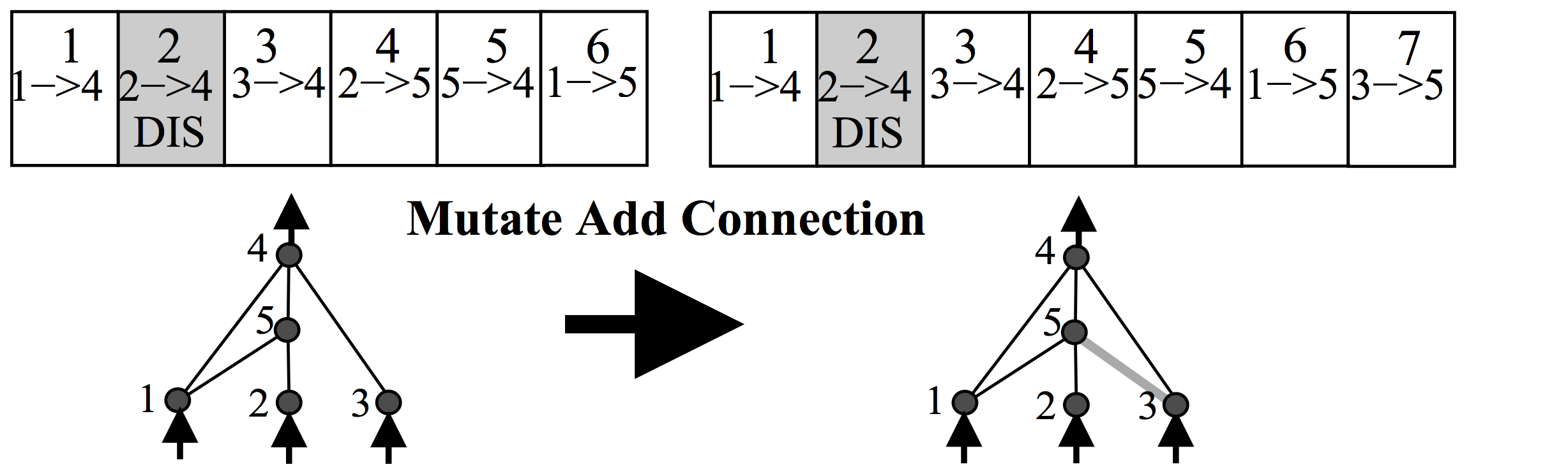
There is also some probability that a new connection will get created in the same mutation operation, like the below:

Each neuron and connection in the entire population is unique, and assigned a unique integer label. So each network is simply just a list of connections, along with the weight for those connections. Note that two different networks can have a similar connection, but the weights for each network will generally be different.

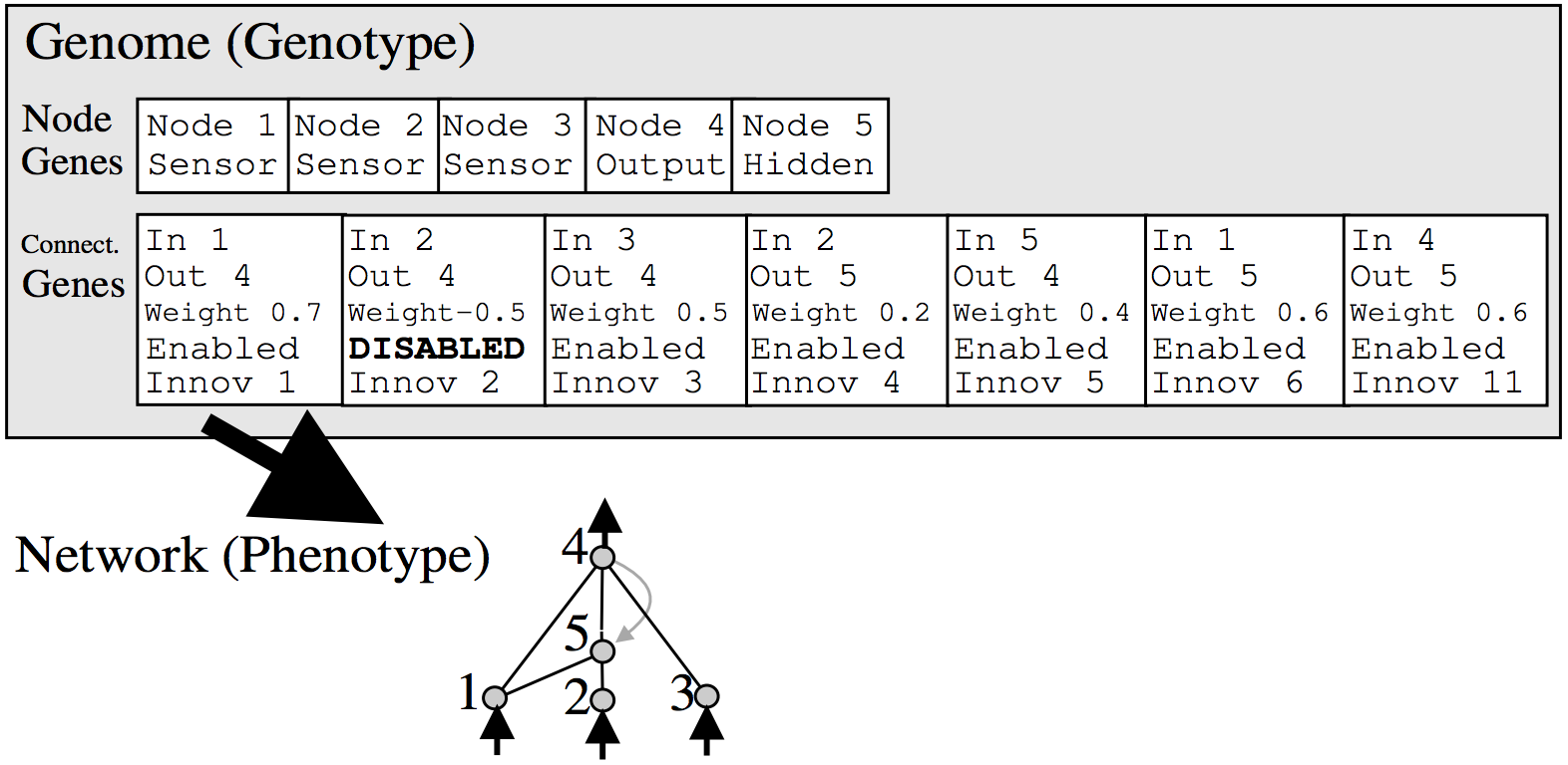
Because each neuron and each connection is globally unique, it becomes possible to merge two different networks, to produce a new network. This is how the crossover operation is done in NEAT:

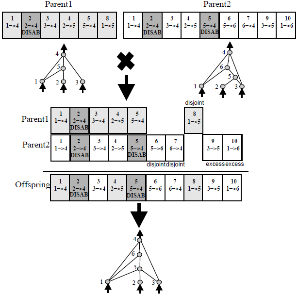
All diagrams from original NEAT paper, highly recommended reading!

The crossover operation is quite powerful. If we have a network that is good at some sub task, and another network that is good at some other sub task, we may be able to breed an offspring network that can potentially be good at combining both skills and becoming much better than both parent networks at performing a bigger task.

Now that the mutation and crossover operations are defined, we can simply use the genetic algorithm I described earlier to discover new networks by evolving them through many generations! We are not there yet, however, as there is more than these genetic operators in the NEAT algorithm.

Speciation

In evolutionary computing, speciation is the idea to group the population of genes into different species consisting of similar members of the population. The idea is to give certain members of the population, who may not be the best at performing the task, but look and behave very different than those who are currently the best, more time to evolve to their full potential, rather than to kill them off at each generation.

Imagine an isolated island populated by wolves and penguins only. If we let things be, the penguins will be dead meat after the first generation and all we would be left with are wolves. But if we create a special no kill zone on the island where wolves are not allowed to kill penguins once they step inside that area, a certain number of penguins will always exist, and have time to evolve into flying penguins that will make their way back to the mainland where there’s plenty of vegetation to live on, while the wolves would be stuck forever on the island. It is also possible for some weird wolf with an identity crisis to fall in love with a penguin and start a family together in that zone, and so we may also end up with flying wolf-penguins that will eventually dominate the mainland. Speciation is a powerful concept in artificial evolution.

For a more concrete example, consider the earlier example about the 100 set of weights, and imagine if we modify the algorithm from only keeping the best 20 and getting rid of the rest, to first grouping the 100 weights into 5 groups according to the similarity by, say, using euclidean distance between their weights. Now that we have 5 groups, or species, of 20 networks, for each group we would keep only the top 20% again (so we keep 4 set of weights for each species), and get rid of the remaining 16. From there, we can either decide to populate the remaining 16 by crossover-mutating the 4 remaining members of each species, or from the entire set of surviving members in the larger population. By modifying the genetic algorithm this way to allow speciation, certain types of genes have the time to develop to their full potential, and also the diversity will lead to better genes that incorporate the best of different distinct types of species. Without speciation, it is easy for the population to get stuck at a local optimum.

The NEAT paper also defined a method for speciation. It defined a distance operator to measure how different one network is to another network. Basically, it counts the number of connections that are not shared by the two networks, and of the connections that is shares, it measures the difference in the weights inside the common connections, and the distance between two networks is a linear combination of these factors. Once we can calculate the distance between each network in our population, NEAT prescribes a formula to group networks that are within a certain distance together to form a species, or a sub population. The paper lists some ideas about how to deal with the different species, and when to cross-breed species and make certain species go extinct if you are interested to read further into the details.

My personal take is that while the concept of speciation is important, the exact implementation on how to achieve speciation is quite flexible and there’s no de facto correct approach. In my implementation of NEAT for this demo, I actually disregarded NEAT’s speciation method, and ended up using the K-Medoids algorithm to divide our population of 100 networks into 5 clusters based on the calculated distance between the networks. We cannot use K-means clustering because we only know the distance between each network, rather than the exact location in hyper dimensional space. This approach ended up working quite well, and seems more elegant and simple to me for the purposes of the simple classification task in this demo.

Backprop NEAT

Forget Torch, Tensorflow, and Theano. I decided to implement Backprop NEAT in Javascript, because it is considered the best language for Deep Learning according to the Data Science Dojo.

I implemented the genetic operators portion of NEAT for an earlier project called Neurogram, which allows the user to interactively evolve a population of neural network using the NEAT-style crossover and mutation operators, for the purpose of creating genetic art. To generate a picture, the coordinates of every pixel in that picture will be the inputs to the neural network, and the outputs will be the colour for that very pixel. The more complicated the network, the more detailed the resulting picture would be.

In our implementation of NEAT, I allow for many types of activation functions, represented as different colours in a neural network. Below is a legend for the different activation functions:

The add operator does nothing to the input (which is the weighted sum of outputs of incoming connections), while the mult operator would multiple all the weighted inputs together. By allowing a sinusoidal operator, the network can produce repetitive patterns in the output. The square and abs operators are useful for generating symmetries. Gaussian operator can be helpful to draw one-off clustered regions.

In some sense, the classification problem in TensorFlow Playground can be regarded as a subset of image generation. Each datapoint in the training set corresponds to a class (zero or one), and each datapoint has an (x, y) coordinate. If we modify the art-generation program to output a real number between zero and one, rather than three colour channels, we can try to attempt to get the art-generation program to just draw a monotone picture, where the regions in the monotone picture with intensities below 0.5 will correspond to a prediction of zero and the regions above 0.5 will correspond to a prediction of one.

So it was fairly straightforward to modify the Neurogram NEAT code from image-generation to performing a classification task. The only thing we need to do is to implement the genetic algorithm portion of NEAT along with speciation, so that networks are specifically evolved to fit the training data, rather than generate fancy art.

Since my NEAT implementation works by describing a neural network that is ultimately built as a computation graph that can be processed by recurrent.js, we will also be able perform back propagation and optimise the weights of each individual neural network architecture to best fit the training data. This way, NEAT is strictly responsible for figuring out new architectures, while backprop can try to determine the best set of weights for each architecture that NEAT comes up with. In the original NEAT paper, NEAT is also used to figure out the weights as well using the genetic algorithm operations but I think this is not efficient at all, especially when we know backprop is a superior method for figuring out weights for a simple classification problem. In my implementation, I also incorporate a L2 regularisation term for the weights when performing backprop on each network. In the future, it is also possible to implement other techniques such as dropout.

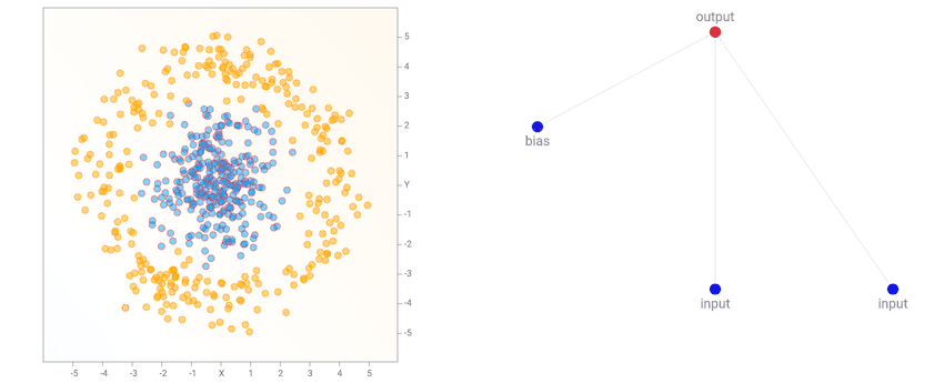
At the beginning, the population of networks will start off looking very simple and minimal, like the one below. Note that for this demo, the output neuron is also a sigmoid operator since we are classifying classes labelled as zero or one. So basically the first generation of networks are all logistic regression networks with a different set of random initial weights.

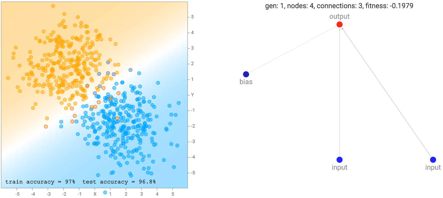
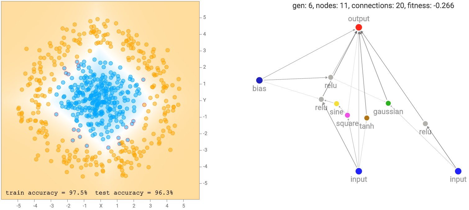
This simple network of just a linear combination of the coordinates into a sigmoid layer will just divide the plane into a line like the diagram above. The region of the output that is close to zero will be painted orange. The region close to one will be painted blue, and the region between zero and one will be blended between the two colours and will be exactly white at 0.5. We see that when the dataset is the two gaussian clusters, the simplest default network will perform quite well already. In fact, we start off with an initial population of 100 simple networks with pure random weights, and before performing any backprop or genetic algorithm is performed on the population, the very best network in the population will already be good enough for this type of dataset.

When evaluating each network, we need to assign each network with a fitness score on how good it is, so we can rank them in the genetic algorithm. In addition to seeing how well each network fits the training data, using maximum likelihood, the number of connections would also affect the fitness score of the network. We would prefer a simpler network over a more complicated network, if they achieve the same regression accuracy, and in some cases we would even prefer a much simpler network over a very complicated one even if the simpler one fits the training data less accurately. To achieve this, I multiply the fitness score by a factor that grows in proportion to the square root of the number of connections.

A network with more connections will have a fitness that is more negative than a network with less connections. I used the square root function because I feel that a network with 51 connections should be treated about the same as a network of 50 connections, while a network with 5 connections should be treated very differently than a network with 4 connections. Other concave utility functions may achieve the same effect. In a way, like the L2 regularisation on weights, this type of penalty is a form of regularisation on the neural network structure itself.

After a few generations of NEAT evolution steps along with performing backprop on each network prior to calculating the fitness score, we end up with some networks that attempt to fit the training data:

More complicated datasets, such as the spiral dataset will require more complicated networks to fit the training data.

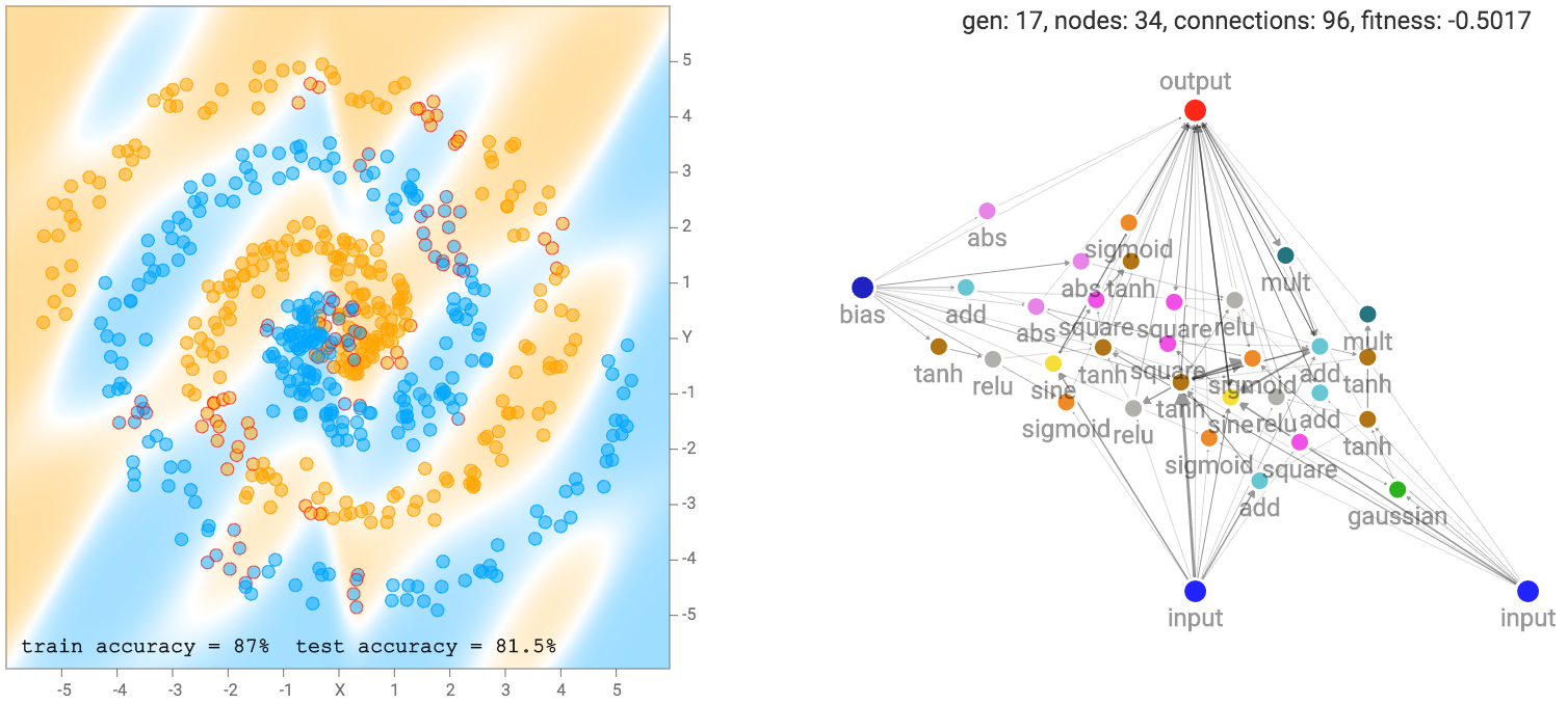
As mentioned earlier, our networks are not made of many structured layers of neurons, and each neuron can connect to any other neurons in the network. Therefore, sometimes even recurrent loops can be formed, such as when the output connection connect back into the hidden neurons. This presents a problem for us when deciding how to traverse the neural network.

For conventional feed-forward neural network in TensorFlow Playground, it is possible to write down in one line of math describing the output as a nested set of functions of the inputs, such as $output = f_1\left( w_1 f_2\left( w_0x + b_0 \right) + b_1 \right)$ for a 2 layer feed forward net, or even $output = f_1\left( w_1x + w_2 f_2\left( w_0x + b_0 \right) + b_1 \right)$ for a 2 layer ResNet. So it is possible to determine the value of the output exactly for every input for these feed forward architectures. However, for a large network produced by NEAT, with many loopy recurrent connections, it might be extremely difficult, or even not possible to express the output as a function of the input we can calculate in one step.

To find the output, we can only propagate every connection together one step at a time, so if the shortest distance between input x and the output consists of 3 connections, then it would take at least 3 steps to obtain an output value that depends on the input, otherwise the output value would be zero. After getting the output, we can use backprop in a way like backpropagation through time when training recurrent networks. The output signal will also be a function of time, or rather a function of how many steps we propagate the network by. The question is when do we stop propagating the signal forward for the purpose of recording the value of the output for use in classification? I have done some thinking about this topic and wrote down my thoughts in an earlier blog post. In the end I opted for the second method to stop when each neuron has been touched at least once, and I think that is a good balance between the options I have.

Evolution Process

In my implementation, I keep a fixed population size of 100 networks. As discussed earlier, I used K-Medoids algorithm to fix the number of sub populations to 5, so the entire population will be clustered into 5 sets of 20 networks that are similar to each other.

In the evolution step, the next generation of each sub network will be created by randomly choosing two networks from the previous generation in the same sub network (it can be the same network chosen twice), weighted by a probability porportional to the fitness score, so better scoring networks will have a higher likelihood of getting chosen to mate and producing offsprings for the next generation. The crossover + mutation genetic operators in NEAT will be applied in this step, so the offsprings in the next generation will likely have on average more neurons and connections compared to the previous generation. This is where new types of activation functions from different neuron types will be experimentally chosen for the next generation to see if they will improve the network.

But sometimes the next generation does not really offer any improvement at all compared to the current generation, and if anything, all the new neurons and connections can be useless for the task at hand. To counter this, I also keep the very best 10 networks from the previous generation and store them in a special hall of fame gene pool to preserve for the next generation so the best of each generation will be cloned for the future, just in case their kids all turn out dumber than their parents. It is unlikely that Michael Jordan’s son will be better than Michael Jordan at basketball. In this world, you may need to compete against your parents in their prime.

Before calculating the fitness score of each network, back propagation will be performed for each network to optimise their weights. By default, each network will be backpropped 600 times. Afterwards, their logistic regression error will be combined with a factor to penalise for the number of connections to compute the fitness score of each network. The fitness score will be used again in the next evolution process.

After every generation of evolution, there is a 50% chance that we will force the poorest performing species to go extinct and kill off all 20 of its members. To fill the gap of the 20 new spots available, we allow the best performing species from the previous generation to produce another 20 additional offsprings. If the penguins don’t learn to fly over time, we will let the wolves in. This will lead to the best performing species to be forked into two sub species and developing in potentially different directions afterwards.

Using the Demo

Okay, with the details of genetic algorithms, NEAT, and backprop out of the way, we can finally discuss how to actually use this demo and explore the different options.

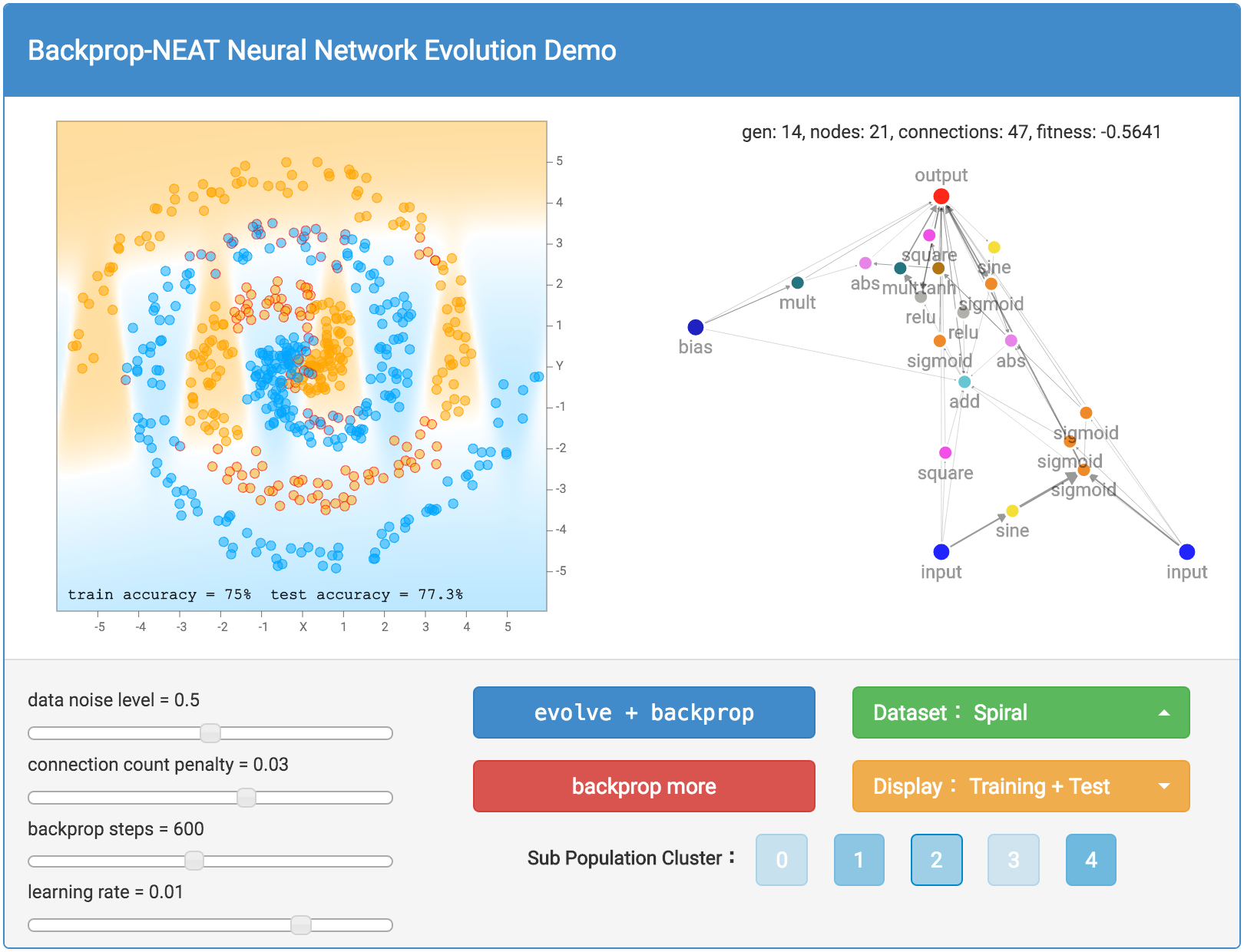
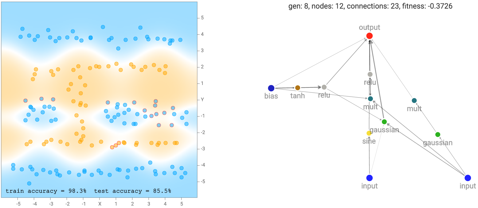
First, we can choose a dataset to play with by selecting one via the green button. I’ve mirrored the datasets used in the TensorFlow Playground demo so you can compare results if you want. There’s the small circle inside a big circle dataset, a XOR dataset, a dataset composed of 2 gaussian clusters, and a spiral dataset that is the most challenging. The amount of randomness of each dataset can be controlled using the data noise level sliding bar on the left. You can also choose to reset and regenerate your dataset at anytime. I’ve also put in a custom dataset mode so you can tap in your own dataset with your mouse or trackpad.

Half of the data generated will belong to the training set and half in the test set. You can use the orange button to choose to which sets you want displayed.

Custom dataset entry. The more datapoints the better.

The magic happens with the blue evolve + backprop button. This button will evolve the entire generation of 100 networks by one generation, described in the previous section, and then perform backprop on each network in the new generation right afterwards. Sometimes you may want to experiment with backpropping the networks further, if you think they haven’t reached their local optimums yet, as this may be the case for networks that have grown very large. So I included a red backprop more button to allow for pure back propagation, and no evolution to take place. In addition, we can control how many steps we backprop by each time, and also the learning rate by adjusting the corresponding slider bars.

After you hit either the evolve + backprop or backprop only button, the network with the very best fitness score will be graphed out with all its neurons and connections onto the right side of the screen. A thicker connection line means the absolute value of the weight is larger. The classification regions, and classification accuracy will also be calculated and displayed on the left side of the screen. In addition to drawing the classification regions, mispredicted samples will have a small red circle surrounding the datapoint to indicate prediction errors. The generation number, neuron count and connection count, and the fitness score of the best network will be printed above the network. As explained earlier, the fitness score also depends on a connection count penalty factor, and the size of this factor can be controlled by a slider bar on the bottom left.

If you wish to see not just the very best network in the population, there is also the option to see the best network in each of the 5 sub populations. There is a button for each sub population cluster, and if you click on one of them, you will be able to bring up and display the best network of that sub population and all the associated information will be based off that network. This will allow you to see the different structures from different species and appreciate the (forced) diversity in the population. By default, the very best sub population, therefore the best network will be selected for display. The relative shading of the colours for the sub population buttons is based on the relative fitness scores for the best members of each sub population. The more solid the colour, the stronger that sub population will be relative to other sub populations.

Results

In the original TensorFlow Playground demo, users get to cheat and use predefined features, such as squaring the inputs, multiplying them, or putting them through a sinusoid, and then feeding in the input and all these hand-engineered pre-processed features into a multi-layer neural network. This has an advantage for a human to visually identify features in the dataset, and pick good features to calculate to simplify the task of the neural network. For example, if the dataset is the small circle inside the big circle, we know that the decision boundary is simply the radius, or even the square of the radius, from the origin, so by squaring both inputs first, most of the work has already been done for the network.

What I’m interested to see is for the genetic algorithm to discover these features by itself via the evolution process, incorporate these feature calculations into the actual neural network via the extra set of available activation functions, and not rely on human engineering. So the raw inputs to each NEAT network will only be the x and y coordinates, and a bias value of 1. Any features, such as squaring the data, or multiplying them, or putting them through a sinusoidal gate, will have to be discovered by the algorithm.

I noticed that for the the two circle data set, it is more likely that the final network consists of many sinusoidal, square or abs activation gates, which makes sense given the symmetry of the dataset. For the XOR dataset, there tends to be more relu activations, which is required to produce decision boundaries that are more or less straight lines with sharp corners.

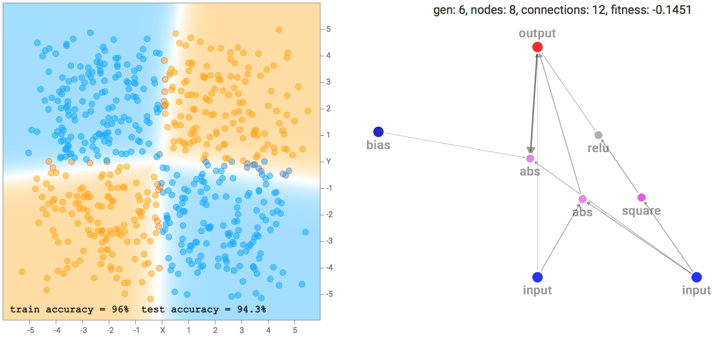XOR Dataset Solution Example

One of the more interesting things I noticed is that networks that backprop well will tend to be favoured in the evolution process, compared to nasty networks with gradients that blow up, since a network with blown up weight values will likely give rubbish classification results that will result in a poor fitness score. Setting a low number of backprop steps, or a large learning rate, may lead the genetic algorithm to produce different types of network that will perform better in those environments.

So even if there exists a set of weights for a certain network that can fit the training data exactly, if the backprop conditions does not allow that network to learn that set of weights, it may end up being discarded by evolution. Maybe an analogy in life would be that people with extrodinarily high IQ’s may never reach their full potential if they live in a very harsh environment during a barbaric era that favour raw physical strength and a desire to prey on the weak. Or in modern times, people with high raw intelligence also might fail to get ahead if they lack the people skills to influence their peers in society to accept their ideas.

Future Work

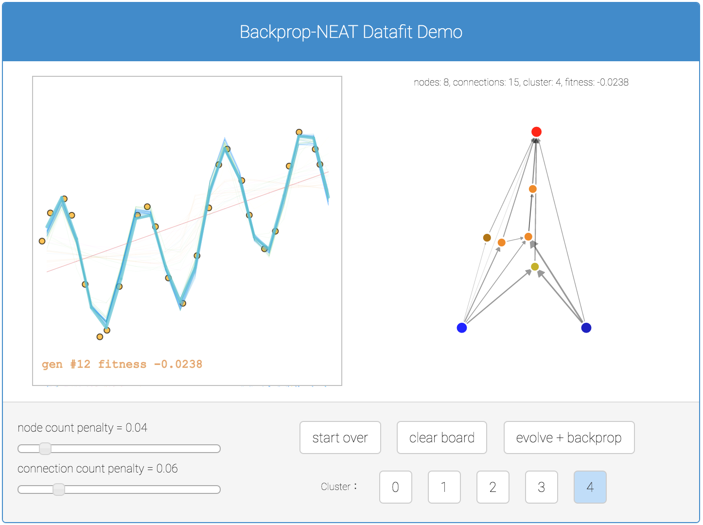
In addition to classification problems, I have created a similar demo earlier to get Backprop NEAT to work on regression problems. Below is a simple demo for regression if you are interested. In this demo, all five sub population results are plotted in the canvas for better comparison.

One of the tasks I am interested to see neuroevolution work on is to use evolution to discover new types of small neural network building blocks, such as LSTM blocks, that are often repeated in a much larger deep neural network, or a recurrent neural network. Given a certain deep learning task, and a large number of GPUs (that are becoming more affordable every few months), perhaps in the future it can be feasible to train 100 deep networks in parallel, a few dozen times, based on an evolving small building block neural network component, and see if new novel small network blocks can be discovered that are very good at solving certain problems.

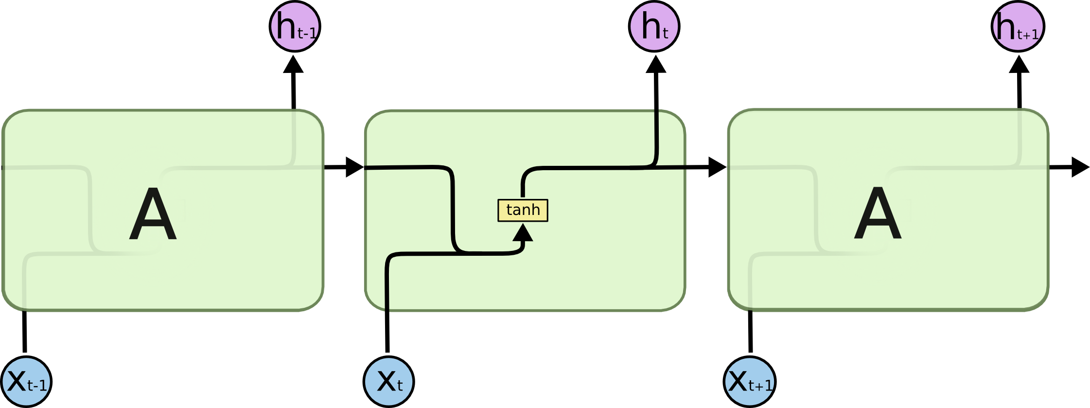Perhaps “A” can be evolved? (Source: Colah’s blog post on LSTMs)

Thanks to the many friends who helped me test drive the neural network evolution playground demo earlier, and for the valuable feedback used to finetune and improve it.

Citation

If you find this work useful, please cite it as:

@article{ha2016backpropneat,
  title   = "Neural Network Evolution Playground with Backprop NEAT",
  author  = "Ha, David",
  journal = "blog.otoro.net",
  year    = "2016",
  url     = "https://blog.otoro.net/2016/05/07/backprop-neat/"
}